Download
1 / 9
110 likes | 415 Vues
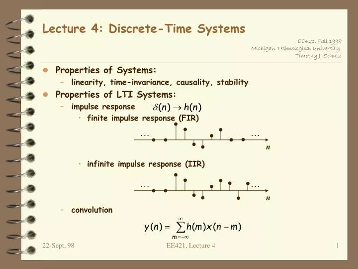
n. n. Lecture 4: Discrete-Time Systems . Properties of Systems: linearity, time-invariance, causality, stability Properties of LTI Systems: impulse response finite impulse response (FIR) infinite impulse response (IIR) convolution. Processing Methods.

E N D
n n Lecture 4: Discrete-Time Systems • Properties of Systems: • linearity, time-invariance, causality, stability • Properties of LTI Systems: • impulse response • finite impulse response (FIR) • infinite impulse response (IIR) • convolution EE421, Lecture 4
Processing Methods • Block processing: output values are computed by processing an entire block of input values. • non real-time processing • Sample processing: output values are computed by processing input samples one at a time. • real-time processing EE421, Lecture 4
Processing Methods • block processing EE421, Lecture 4
+ + + Processing Methods • sample processing output state variables x(n) y(n) a0 a1 a2 a3 r e g r e g r e g w1 w2 w3 EE421, Lecture 4
FIR Filters • Impulse response extends only over a finite time: • filter order = M • convolution equation: filter coefficients, filter weights, filter taps causal system EE421, Lecture 4
FIR Filters • Examples • y(n) = 2x(n) + 3x(n-1) + 5x(n-2) + 2x(n-4)impulse response = {. . ., 0, 0, 2, 3, 5, 0, 2, 0, 0, . . .} • y(n) = (1/4)x(n+1) + (1/2)x(n) + (1/4)x(n-1)impulse response = {. . ., 0, 0, 1/4, 1/2, 1/4, 0, 0, . . .} n=0 n=0 EE421, Lecture 4
IIR Filters • Impulse response extends over an infinite time: • we cannot approach this in the same manner as an FIR filter • IIR filters cannot, in general, be computed! • we restrict our attention to systems described by difference equations: y(n) = y(n-1) + 2y(n-2) + x(n) - x(n-1) a0y(n) + a1y(n-1) + … + aMy(n-M) = b0x(n) + b1x(n-1) + … + bLx(n-L) EE421, Lecture 4
IIR Filters • Examples: • y(n) = ay(n-1) + x(n) • impulse response: h(n) = ah(n-1) + d(n) • h(n) = anu(n) • y(n) = ay(n-2) + x(n) • impulse response: h(n) = ah(n-2) + d(n) • h(n) = an/2, if n is even; h(n) = 0 otherwise EE421, Lecture 4
IIR Filters • Examples: • y(n) = ay(n-1) + x(n) + x(n-1) • impulse response: h(n) = ah(n-1) + d(n) + d(n-1) • h(n) = 1 if n=0, h(n) = an-1(1+a)u(n) otherwise EE421, Lecture 4