Download
1 / 27
270 likes | 485 Vues
Coastal upwelling and satellite observations within the EU Marine Strategy Framework Directive Francesco Bignami, Eleonora Rinaldi, Rosalia Santoleri CNR-ISAC UOS Roma via Fosso del Cavaliere 100 00133 Roma Italy Ph.: +39 06 4993 4634 e-mail: f.bignami@isac.cnr.it.

E N D
Coastal upwelling and satellite observations within the EU Marine Strategy Framework DirectiveFrancesco Bignami, Eleonora Rinaldi, Rosalia Santoleri CNR-ISAC UOS Roma via Fosso del Cavaliere 100 00133 Roma Italy Ph.: +39 06 4993 4634 e-mail: f.bignami@isac.cnr.it
Fluid mechanics equations (Newtonian fluid, e.g. air, water) • Eq. motion (which principle?), three equations, for u, v, w, in x, y, z directions respectively Continuity (which principle?) eq. Incompressible fluid? Eq. of state Heat Eq. Salinity Eq. + what? (to define system, e.g. to make a model work?) + initial and boundary conditions!! NOTE: stuff in red indicates a question for you to answer http://oceanworld.tamu.edu/resources/ocng_textbook/chapter07/chapter07_01.htm http://ocw.mit.edu/courses/earth-atmospheric-and-planetary-sciences/12-333-atmospheric-and-ocean-circulations-spring-2004/
Evaluating the terms of an equation: scaling (example: x momentum equation) NOTE: ALL equations are scaled in fluid dynamics work . • introduce typical values so that velocity u=Uu*; horizontal (x,y) space (x,y)=L(x*,y*); vertical (z) space z=Wz*, time t=Tt* • obtain new equation with magnitude (e.g. U) and variability (e.g. u*) • “starred” variables of order 1 • e.g. if u = (-0.2,0.2) m/s and we set U = 0.2 m/s then u* = O(1) NON-DIMENSIONAL • (after dividing by fU... TRY THIS AT HOME! Substituteu=Uu*, etc. in the eq., divide by fU and obtain new eq.). Find scaling of other equations • http://en.wikipedia.org/wiki/Non-dimensionalization_and_scaling_of_the_Navier%E2%80%93Stokes_equations • http://en.wikipedia.org/wiki/Navier%E2%80%93Stokes_equations
Scaling (cont’d) If we now introduce a few “fluid mechanics numbers” (“magic numbers”): • 1/fT = RoT(temporal Rossby number, in honor of Carl-Gustav Arvid Rossby, Swedish) • U/fL = Ro(Rossby number) • /fH2 = EkV(vertical Ekman number, in honor of Vagn Walfrid Ekman, Swedish) • /fL2 = EkH (horizontal Ekman number) THEN ALL EQUATIONS OF FLUID DYNAMICS (OR ANY OTHER PROCESS EXPRESSIBLE BY MEANS OF A SYSTEM OF EQUATIONS) MAY BE SCALED IN THIS WAY, SO THAT: • THEY MAY BE SIMPLIFIED BY DISCARDING TERMS WHICH ARE SMALL, GIVEN THE TYPICAL VALUES OF THESE “MAGIC NUMBERS” IN THE PHENOMENON UNDER STUDY • ONE MAY MAKE LAB MODELS OF VERY LARGE OR VERY SMALL SCALE PHENOMENA: IT IS SUFFICIENT THAT LAB HARDWARE RESPECTS MAGIC NUMBER VALUES TYPICAL OF THE PHENOMENON (EG. TANK LENGTH, PUMP CURRENT, ETC. FOR REPRODUCTION OF GULF STREAM) • SAME HOLDS FOR NUMERICAL MODELS (SETTING OF MAGIC NUMBERS IS NECESSARY FOR CORRECT COMPUTER SIMULATION IN LAB TANK) • http://en.wikipedia.org/wiki/Non-dimensionalization_and_scaling_of_the_Navier%E2%80%93Stokes_equations
By the way: T is the typical time for a parcel to cover L (H)with velocity U (W), so: therefore For most ocean problems,L = O(1-1000 km), H = O(10-1000 m), so W is typically 100-1000 times SMALLER than U. • If we concentrate on upwelling events, typically L = O(10-100 km), U = O(0.1 m/s), H = O(100 m), then [withf = O(10-4 s-1), = O(1000 kg m-3), • (eddy) = O(horizontal: 10 – 105 m2 s-1 ; vertical: 10-1 m2 s-1)] we have: • RoT, Ro = 10-1 - 10-2EkV = 10-4 EkH = 10-4 - 10-1 • SO ALL TERMS ARE NEGLIGIBLE WITH RESPECT TO CORIOLIS TERM –v*PRESSURE TERM MUST BE O(1) FOR THE EQUATION TO HOLD! • WE ARE LEFT WITH • ...BUT THIS IS GEOSTROPHIC EQUILIBRIUM, A.K.A. BUT IF WE “THROW EVERYTHING AWAY” EXCEPT CORIOLIS AND PRESSURE TERMS, HOW CAN OUR OCEAN CHANGE IN TIME AND/OR HOW CAN A CURRENT SLOW DOWN (FRICTION)? ALSO, HOW CAN WE HAVE WIND-DRIVEN CURRENTS? http://oceanworld.tamu.edu/resources/ocng_textbook/chapter07/chapter07_01.htm
z L d d - surface Ekman layer (wind stress) H y d • d - bottom Ekman layer (bottom stress) x INDEED, UPWELLING HAS TO DO WITH FRICTION (I.E. WIND-DRIVEN CURRENTS), I.E. EKMAN PHENOMENOLOGY. THEREFORE, FRICTIONAL TERMS MUST BE IMPORTANT (ORDER 1) SOMEWHERE, IF NOT IN THE ENTIRE OCEAN, E.G. IN A SUB-LAYER OF THICKNESS d OF THE WATER COLUMN H SUCH THAT . THAT IS: NEAR THE SURFACE AND NEAR THE BOTTOM d (wind-mixed layer, Ekman influence)
Ekman Layer at the Sea Surface What is it all about? We investigate the effect on the water of a steady surface wind, in the presence of the Coriolis effect... this does NOT happen in a bathtub (why?)! Assumptions: ocean homogeneous in x,y and z, infinite depth, steady state, linearity (i.e. Ro and RoT small), EkV = O(1) (we are looking at what happens in the d layer), so horizontal diffusion not occurring or not important (why?) Equations (momentum, after subtracting geostrophic velocity (ugeo, vgeo) from total velocity Can you obtain them from the general eqs. using the assumptions?): . Boundary conditions Purely geostrophic velocity at depths beyond d (why?) Frictional term (stress) = wind stress at sfc (units?) Wind stress: example of simple parameterization Ekman, V.W. 1905. On the influence of the Earth’s rotation on ocean currents. (1905). Arkiv for Matematik, Astronomi, och Fysik, 2 (11)1–52 Beesley, D., J. Olejarz, A. Tandon and J. Marshall (2008). Coriolis Effects on wind-driven ocean currents (2008). Oceanography, 21(2),72-76. http://oceanworld.tamu.edu/resources/ocng_textbook/chapter09/chapter09_02.htm
Solution (one of the few cases in GFD we have a “pencil and paper” computable solution) (compare to our estimate of “frictionally important layer” d using EkV) Comments: total current u is made of geostrophic + Ekman-frictional components wind stress appears in Ekman current velocity affecting magnitude at all depths ez/d is the “magnitude reduction with depth” part of Ekman current check that velocity tends to geostrophic velocity at depth z • THIS IS (u-ugeo,v-vgeo) NOT TOTAL • CURRENT (u,v) the sin and cos part is the “spiral rotation part” understand iceberg motion now (look carefully!)? Given the figure and eqs., how are the x and y axes located with respect to the wind direction (choose x and y first)? Who did this calculation for the first time? • Vagn Walfrid Ekman (in 1905), to explain why icebergs float at 45° w/respect to the downwind direction, upon Prof. V. F. K. Bjerknes’ request (his PhD tutor). Smart Swedish tutor and smart Swedish student.
Surface Ekman dynamics near a coast – upwelling (Northern Hemisphere case) First, we define Ekman transport, as the water volume moved within surface layer d by the frictional part of the velocity (the same concept holds for bottom Ekman layer) (proportional to wind stress... reasonable!) SFC. SLOPE [THUS GRAD(P), THUS (ugeo, vgeo)] TIME – DEPENDENT JUST AFTER WIND STARTS: MUST CONSIDER AT LEAST (u,v)/t TERMS. SO THE STATIONARY EQUATIONS (GEOSTROPHIC, EKMAN) ARE APPLICABLE AS “SNAPSHOTS” OF THE EVOLVING SITUATION, AND DESCRIBE THE MOST IMPORTANT TERMS AT EACH INSTANT. BUT THE SMALL TERMS ARE THOSE WHO LITTLE BY LITTLE CHANGE THE SYSTEM IN TIME. sea surface wind EQUILIBRIUM CONFIGURATION x (along-shore) coast sfc. Ekman transport (N. Hem.) cross-shore pressure gradient buildup (due to sfc. slope) H L geostrophic current buildup upwelling (colder water) Ekman btm. transport (N. Hem.) z sea bottom y (cross-shore)
Now, that was a nice little story... very neat, homogeneous along-shore, etc. BUT if we start looking at real cases... Bignami et al. (2008) http://www.mbari.org/canon/Images/upwellinggraph.jpg This is quite orderly... ...this a little more complicated... • ... actually a mess! Need full equations because of: • instability occurrence • wind variability (equilibrium not reached) • stratification • variable coastline and bathymetry (points, heads) • Lagrangian model domain: 250 km alongshore, all with same bathymetry as black line above, i.e. off big Sur, CA, USA, i.e. a “constant bathymetry section” coast Bignami, F., E. Böhm, E. D'Acunzo, R. D'Archino and E. Salusti (2008), On the dynamics of surface cold filaments in the Mediterranean Sea, J. Mar. Sys., 74 1-2, 429-442. http://www.mbari.org/canon/Images/upwellinggraph.jp • Lagrangian simulation (Harrison et al., 2014) Harrison, C. S. and D. A. Siegel (2014). The tattered curtain hypothesis revised: Coastal jets limit cross-shelf larval transport . Limnology & Oceanography: Fluids & Environments,4:,50-66. DOI:10.1215/21573689-2689820
Upwelling index with satellite Sea Surface Temperature (SSTindex) (implemented for the Marine Strategy Framework Directive report sheets on Good Environmental Status – Italian seas) Land mask for SST images (0,1 values) Angle of perpendicular to coast map Data: MyOcean multi-sensor optimally interpolated satellite SST (2009-2011, daily; 7 km resolution) Daily SST and monthly SST climatology extracted 49 sections chosen for SSTindex (MSFD work) SST data browsable/available at: http://www.myocean.eu.org/; MSFD stuff at: http://www.msfd.eu/
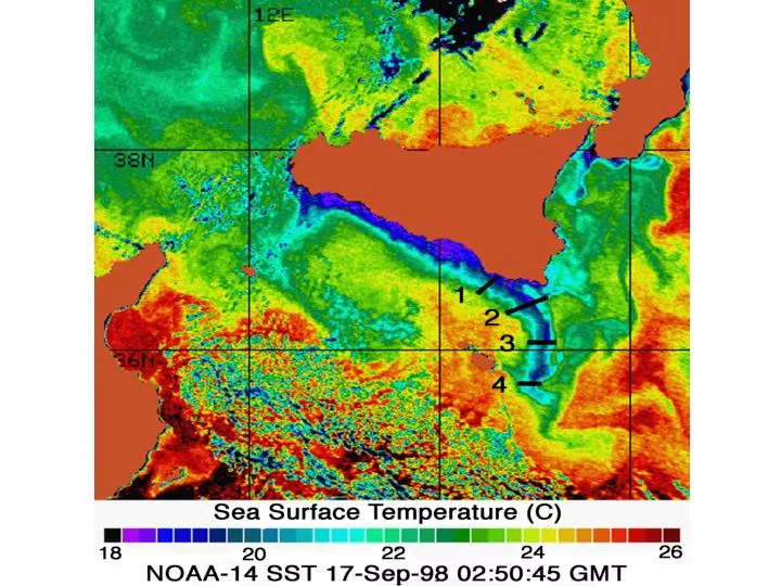
SSTindex (cont’d) Pixels for SSTdayMIN Pixels for SSTdayMAX SSTdaymin max SST grad location SSTdayMIN= minimum SST in the (0, 2*Rd) distance from the coast (red dots) SSTdayMAX= mean SST value relative to all pixels seaward of maximum SST gradient (blue dots) SSTclimMIN and SSTclimMAX = same as SSTdayMINand SSTdayMAX, but of 2009-2011 monthly SST climatology NOTE: SSTclimMIN - SSTclimMAX is subtracted from SSTdayMAX – SSTdayMIN to avoid inclusion of false upwelling due to e.g. riverine cold coastal currents, as in the Adriatic Sea • Demarcq, H., and V. Faure (2000). Coastal upwelling and associated retention indices derived from satellite SST. Application to Octopus vulgaris recruitment. Ocean. Acta, 23, 391-408. • Marine Strategy Framework Directive http://www.msfd.eu/
SSTindex (cont’d) SSTindex frequency= 40% day 2009-2011 (SSTindex threshold under construction... 0.1 adopted by trial and error) Upwelling frequency fSST = 40% indicates that the Sicilian coast is frequently subject to upwelling, in agreement with the well known quasi-permanent upwelling activity there (e.g. Béranger et al., 2004)... SSTindex seems to work! However, to be sure of this we may use another tool: wind. Béranger, K., L. Mortier, G. P. Gasparini,L. Gervasio, M. Astraldi and M. Crépon. (2004). The dynamics of the Sicily Strait: a comprehensive study from observations and model, Deep Sea Res. II, 51, 411–440.
Wind upwelling index: Windex (offshore Ekman transport) Scatterometer multi-satellite winds (2009-2011, 6-hourly wind data, 25 km resol.) (with daily mean winds) then compute wind stress air= 1.2 kg m-3; Cd= 0.0012 for 0 < |Uwind| < 11 m/s and Cd= 0.00049+0.000065 | Uwind | for | Uwind | >11 m/s (Large and Pond, 1981) • Wind data info at: http://podaac.jpl.nasa.gov/dataset/CCMP_MEASURES_ATLAS_L4_OW_L3_0_WIND_VECTORS_FLK • Large, W. G. and S. Pond (1981). Open ocean momentum flux measurements in moderate to strong winds. J. Phys. Ocean., 11, 324-481.
Windex (cont’d) water = 1025 kg m-3 (constant water density... an approximation) f : Coriolis parameter = O(10-4 s-1) at temperate latitudes; k = vertical unit vector; a= 0.4 from Csanady (1982). Surface Ekman transport (compare to UE, VE in slide # 10) is Ekman Transport M is M component parallel to the coast (refer to yellow line perpendicular section found for SSTindex calculations) wind is Ekman Transport component perpendicular to the coast i.e. Windex Upwelling favorable day when Windex > 0 (offshore) for the previous 2 days + magnitude thresholding under construction Csanady, G. T. (1982a): Circulation in the Coastal Ocean. D. Reidel Publishing Co., Dordrecht, Holland, 279 pp. Csanady, G. T. (1982b): On the structure of transient upwelling events. J. Phys. Oceanogr., 12, 84–96. Check out NOAA site for upwelling index off California (e.g. Google “NOAA upwelling”)
Windex (cont’d) SSTindexfrequency= 40% 2009 2010 2011 Frequencies match in some cases such as Mazara (Sicily)... Windexfrequency= 45% 2009 2010 2011 ... but single days have SST-wind index mismatches, so it needs work.
Cosa si vede da satellite (2003) SST chl torbidità
Cosa si vede da satellite (2006) SST chl torbidità
Stz. 9-15 (delta del Po) Po largo
Stz. 9-15 (delta del Po) Po largo Trasmissometro (torbidità)
Discussione • Giustifichiamo la circolazione, visto il vento • Correliamo la circolazione alle oss. Satellite • Considerazioni sulla conservazione della massa • Considerazioni sull’Ekman layer di fondo • Considerazioni sedimentologiche e biologiche