Distributed Systems

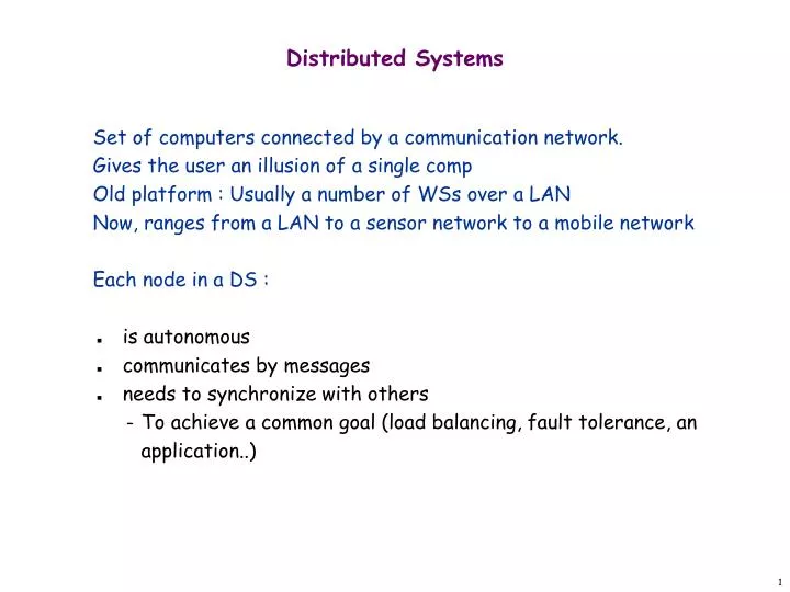
1. Distributed Systems • Set of computers connected by a communication network. • Gives the user an illusion of a single comp • Old platform : Usually a number of WSs over a LAN • Now, ranges from a LAN to a sensor network to a mobile network • Each node in a DS : • is autonomous • communicates by messages • needs to synchronize with others • To achieve a common goal (load balancing, fault tolerance, an application..)

2. Modern Distributed Applications • Collaborative computing • Military command and control • Shared white-board, shared editor, etc. • Online strategy games • Stock Market • Distributed Real-time Systems • Process Control • Navigation systems, Airline Traffic Monitoring (ATM) in the U.S. – largest DRTS Mobile Ad hoc Networks Rescue Operations, emergency operations, robotics Wireless Sensor Networks Habitat monitoring, intelligent farming Grid

3. The Internet (Internet Mapping Project, color coded by ISPs)

4. Distributed Systems: Architecture

5. Issues in Building Distributed Applications • Reliable communication • Consistency • same picture of game, same shared file • Fault-tolerance, high-availability • failures, recoveries, partitions, merges • Scalability • How is the performance affected as the number of nodes increase ? • Performance • What is the complexity of the designed algorithm ?

6. Future : Mobile Distributed (and Real-Time ??)Computing Systems • Wireless data communications • Mobile revolution is inevitable • Two important distributed algorithms Applications : • - Mobile ad hoc Networks (MANETs) • - Wireless Sensor Networks (WSNs) • Can we still apply DS principles ? • Problems : • Location is dynamically changing info • Security issues • Limited storage on mobile hosts

7. Application Areas • These areas have provided classic problems in distributed/concurrent computing: • operating systems • (distributed) database systems • software fault-tolerance • communication networks • multiprocessor architectures

8. Distributed Algorithms : A Perspective (K. Erciyes 2007)

9. A message passing model • System topology is a graph G = (V, E), where • V = set of nodes (sequential processes) • E = set of edges (links or channels, bi/unidirectional) • Four types of actions by a process: • - Internal action -input action • - Communication action -output action

10. Finite State Machines for Modelling Distributed Algorithms • A Finite State Machine is a 5-tuple : • I : Set of Inputs • S : Set of States • S0 : Initial state • G : S X I -> S State Transfer Function • O : Set of outputs • Ç : S X I -> O Output Function

11. FSMs • Moore FSM : Output is dependent on the current state • Mealy FSM : Output is dependent on the input and the current state. It usually has less states than Moore FSM • A Moore FSM example : Parity Checker

12. Process FSMs Each process is a FSM. They execute the same FSM code but may be in different states.

13. Distributed Algorithms Models • Interprocess Communication method: accessingshared memory, point-to-point or broadcastmessages, or remote procedure calls. • • Timing model: synchronous or asynchronousmodels. • • Failure models: reliable or faulty behavior;Byzantine failures (failed processor can behavearbitrarily).

14. We assume • A distributed network—Modeled as a graph. Nodesare processors and edges are communication links. • • Nodes can communicatedirectly(only) with theirneighbors through the edges. • • Nodes haveuniqueprocessor identities. • • Synchronous model: Time is measured in rounds(time steps). • • One message (typically of size O(log n)) can besent through an edge in a time step. A node cansend messages simultaneously through all its edgesat once in a round. • • No failure of nodes or edges. No malicious nodes.

15. Distributed Tree based Communication Algorithms • Broadcast • Convergecast • BFS Tree Construction

16. Broadcast • Broadcasting means sending a message from a source node to all other • nodes of the network. • Two basic broadcasting approaches are flooding and • spanning tree-based broadcast. • Flooding: • A source node s wants to send a message to all • nodes in the network.s simply forwards the message over all its edges. • Any vertex v!= s, upon receiving the message for • the first time (over an edge e) forwards it on every • other edge. • Upon receiving the message again it does nothing.

17. Broadcast • Definition 2.2.1 [Broadcast]: A broadcast operation is initiated by a single processor, the source.The source wants to send a message to all other nodes in the system. • Definition 2.2.2[Distance, Radius, Diameter]: • The distance between two nodes u, v in anundirected graph is the number of hops of a minimum path between u and v. • The radius of anode u in a graph is the maximum distance between u and any other node. The radius of agraph is the minimum radius of any node in the graph. • The diameter of a graph is themaximum distance between two arbitrary nodes.

18. Broadcast • Theorem 2.2.1[Lower Bound]: The message complexity of a broadcast is at least n-1. Theradius of the graph is a lower bound for the time complexity. • Proof: Every node must receive the message. • Remarks: • • You can use a pre-computed spanning tree to do the broadcast with tight messagecomplexity. • • If the spanning tree is a breadth-first spanning tree (for a given source), then also thetime complexity is tight. • Definition 2.2.3: A graph (system/network) is clean if the nodes do not know thetopology of the graph. • Theorem 2.2.2[Clean Lower Bound]: For a clean network, the number of edges is a lowerbound for the broadcast message complexity. • Proof: If you do not try every edge, you might miss a whole part of the graph behind it.

19. Flooding • Algorithm 2.2.1[Flooding]: The source sends the message to all neighbors. Each nodereceiving the message the first time forwards to all (other) neighbors. • Remarks: • • If node v receives the message first from node u, then node v calls node u “parent”.This parent relation defines a spanning tree T. If the flooding algorithm is executed ina synchronous system, then T is a breadth-first spanning tree (with respect to the root). • • More interestingly, also in asynchronous systems the flooding algorithm terminatesafter r time units, where r is the radius of the source. (But note that the constructedspanning tree needs not be breadth-first.)

20. Flooding Analysis • Theorem : The message complexity of flooding is(|E|) and the time complexity is (D), where D isthe diameter of G. • Proof. The message complexity follows from the factthat each edge delivers the message at least once andat most twice (one in each direction). To show the time complexity, we use induction on t to show that aftert time units, the message has already reached every • vertex at a distance of t or less from the source

21. Broadcast Over a Rooted Spanning Tree • Suppose processors already have information about a rooted spanning tree of the communication topology • tree: connected graph with no cycles • spanning tree: contains all processors • rooted: there is a unique root node • Implemented via parent and children local variables at each processor • indicate which incident channels lead to parent and children in the rooted spanning tree

22. Broadcast Over a Rooted Spanning Tree: A Simple Algorithm • 1. root initially sends msg to its children • 2. when a node receives msg from its parent • sends msg to its children • terminates (sets a local boolean to true) • Synchronous model: • time is depth of the spanning tree, which is at most n - 1 • number of messages is n - 1, since one message is sent over each spanning tree edge • Asynchronous model: • same time and messages

23. Tree Broadcast • Assume that a spanning tree has been constructed. • Theorem . For every n-vertex graph G with aspanning tree T rooted at r0, the message complexityof broadcast is n−1 and time complexity is depth(T). • A broadcast algorithm can be used to construct aspanning tree in G. • The message complexity of broadcast isasymptotically equivalent to the message complexityof spanning tree construction. • Using a breadth-first spanning tree, we get the • optimal message and time complexities for broadcast.

24. Convergecast • Again, suppose a rooted spanning tree has already been computed by the processors • parent and children variables at each processor • Do the opposite of broadcast: • leaves send messages to their parents • non-leaves wait to get message from each child, then send combined info to parent

25. f a b c d e c,f,h b,d f,h d e,g g h g h Convergecast solid arrows: parent-child relationships dotted lines: non-tree edges

26. Finding a Spanning Tree Given a Root • a distinguished processor is known, to serve as the root • root sends M to all its neighbors • when non-root first gets M • set the sender as its parent • send "parent" msg to sender • send M to all other neighbors • when get M otherwise • send "reject" msg to sender • use "parent" and "reject" msgs to set children variables and know when to terminate

27. c b b c a a d f f d e e g h g h Execution of Spanning Tree Alg. Both models: O(m) messages O(diam) time Asynchronous: not necessarily BFS tree Synchronous: always gives breadth-first search (BFS) tree

28. Distributed Path Traversals • Distributed BFS Algorithms • Distributed DFS Algorithms

29. Bellman-Ford BFS Tree • Algorithm : Use a variant of the flooding algorithm. Each node and each message store an integer which corresponds to the distance from the root. The root stores 0, every other node initially ∞. The root starts the flooding algorithm by sending a message “1” to all neighbors. • A node u with integer x receives a message “y” from a neighbor v: if y < x then node u stores y (instead of x) and sends “y+1” to all neighbors (except v).

30. Distributed Bellman-Ford BFS Algorithm • 1. Initially, the root sets L(r0) = 0 and all other • vertices set L(v) = 1. • 2. The root sends out the message Layer(0) to all • its neighbors. • 3. A vertex v, which gets a Layer(d) message • from a neighbor w does: • If d + 1 < L(v) then parent(v) = w; • L(v) = d + 1; • Send Layer(d + 1) to all neighbors except w. • Time complexity: O(D). • Message Complexity: O(n|E|).

31. Analysis • Analysis of Algorithm: The time complexity of Algorithm 3.10 is O(D), the message complexity is O(n|E|), where D is the diameter of the graph. • Proof: We can prove the time complexity by induction. We claim that a node at distance d from the root has received a message “d” by time d. The root knows by time 0 that it is the root. A node v at distance d has a neighbor u at distance d-1. Node u by induction sends a message “d” to v at time d-1 or before, which is then received by v at time d or before. • Message complexity : A node can reduce its integer at most n-1 times; each of these times it sends a message to all it neighbors. If all nodes do this we have O(n|E|) messages.

32. Remarks • There are graphs and executions that produce O(n|E|) messages. • How does the algorithm terminate? • Algorithm 3.8 has the better message complexity; algorithm 3.10 has the better time complexity. The currently best known algorithm has message complexity O(|E|+n log3 n) and time complexity O(D log3 n). • How do we find the root?!? Leader election in an arbitrary graph: FloodMax algorithm. Termination? Idea: Each node that believes to be the “max” builds a spanning tree… (More for example in Chapter 15 of Nancy Lynch “Distributed Algorithms”)

33. Distributed DFS • Distributed DFS algorithm: There is a single message called the token • 1. Start exploration (visit) at root r. • 2. When v is visited for the first time: • 2.1 Inform all neighbors of v that v has been visited. • 2.2 Wait for acknowledgment from all neighbors. • 2.3 Resume the DFS process. • The above algorithm ensures that only tree edges • are traversed. • Hence time complexity is O(n). • Message complexity is O(|E|).

34. Distributed Minimum Spanning Tree Algorithms

35. Applications • MST is fundamental problem with diverse applications. • Network design • telephone, electrical, hydraulic, TV cable, computer, road • Approximation algorithms for NP-hard problems • traveling salesperson problem, Steiner tree • Indirect applications • max bottleneck paths • LDPC codes for error correction • image registration with Renyi entropy • learning salient features for real-time face verification • reducing data storage in sequencing amino acids in a protein • model locality of particle interactions in turbulent fluid flows • autoconfig protocol for Ethernet bridging to avoid cycles in a network • Cluster analysis.

36. Greedy Algorithms • Kruskal's algorithm. Start with T = . Consider edges in ascending order of cost. Insert edge e in T unless doing so would create a cycle. • Reverse-Delete algorithm. Start with T = E. Consider edges in descending order of cost. Delete edge e from T unless doing so would disconnect T. • Prim's algorithm. Start with some root node s and greedily grow a tree T from s outward. At each step, add the cheapest edge e to T that has exactly one endpoint in T. • Remark. All three algorithms produce an MST.

37. Chang-Robert’s algorithm {The root is known} Uses signals and acks, similar to the termination detection algorithm. Uses the same rule for sending acknowledgment. Distributed Spanning tree construction For a graph G=(V,E), a spanning tree is a maximally connected subgraph T=(V,E’), E’ E,such that if one more edge is added, then the subgraph is no more a tree. Used for broadcasting in a network. Question:What if the root is not designated?

38. program probe-echo define N : integer (no. of neighbors) C, D : integer; initially parent :=i; C=0; D=0; {for the initiator} send probes to each neighbor; D:=no. of neighbors; do D!=0  echo -> D:=D-1 od {D=0 signals end} { for a non-initator process i>0} do probe parent=iC=0 -> C:=1; parent := sender; ifi is not a leaf -> send probes to non – parent neighbors; D:= no. of non-parent neighbors fi;  echo -> D:=D-1;  probe  sender != parent -> send echo to sender;  C=1  D=0 -> send echo to parent; C:=0; od Chang Roberts Spanning Tree Alg

39. Distributed MST • DefMST Fragment : In a weighted graph G = (V,E,w), a tree T in G is called anMST fragment of G, i there exists an MST of G such that T is asubgraph of that MST. • DefMWOE : An edge e is an outgoing edge of a MST fragment T, iff exactlyone of its endpoints belongs to T. The minimum weight outgoing • edge is denoted MWOE(T). • Lemma : Consider a MST fragment T of a graph G = (V, E,w). Let • e = MWOE(T). Then T U e is a MST fragment as well. • Proof : Let TM be an MST containing T. If TM contains T we are done. • Otherwise, let e’ be an edge that connects T to the rest of TM. • Clearly, e’ is an outgoing edge of T and w(e’)>=w(e).Adding e to TM, creates a graph C with a cycle through e and e’.Discarding e’ from C yields a new T’ M with w(T’ M) >= w(TM).

40. Minimum Spanning Tree • Given a weighted graph G = (V, E), generate a spanning tree T = (V, E’) such that the sum of the weights of all the edges is minimum. • Applications • On Euclidean plane, approximate solutions to the traveling salesman problem, • Lease phone lines to connect the different offices with a minimum cost, • Visualizing multidimensional data (how entities are related to each other) • We are interested in distributed algorithms only The traveling salesman problem asks for the shortest route to visit a collection of cities and return to the starting point.

41. Example

42. Sequential algorithms for MST • Review (1) Prim’s algorithm and (2) Kruskal’s algorithm. • Theorem. If the weight of every edge is distinct, then the MST is unique.

43. GHS is a distributed version of Prim’s algorithm. Bottom-up approach. MST is recursively constructed by fragments joined by an edge of least cost. Gallagher-Humblet-Spira (GHS) Algorithm 3 7 5 Fragment Fragment

44. Challenges Challenge 1. How will the nodes in a given fragment identify the edge to be used to connect with a different fragment? A root node in each fragment is the coordinator

45. Challenges • Challenge 2. How will a node in T1 determine if a given edge connects to a node of a different tree T2 or the same tree T1? Why will node 0 choose the edge e with weight 8, and not the edge with weight 4? • Nodes in a fragment acquire the same name before augmentation.

46. Two main steps • Each fragment has a level. Initially each node is a fragment at level 0. • (MERGE) Two fragments at the same level L combine to form a fragment of level L+1 • (ABSORB) A fragment at level L is absorbed by another fragment at level L’ (L < L’)

47. To test if an edge is outgoing, each node sends a test message through a candidate edge. The receiving node may send accept or reject. Rootbroadcastsinitiate in its own fragment, collects the report from other nodes about eligible edges using a convergecast, and determines theleast weight outgoing edge. Least weight outgoing edge test accept reject

48. Case 1. If name (i) = name (j) then send reject Case 2. If name (i)≠name (j)level (i)  level (j) then send accept Case 3. If name (i) ≠ name (j)  level (i) > level (j) then wait untillevel (j) = level (i). Levels can only increase. Question: Can fragments wait for ever and lead to a deadlock? Let i send test to j Accept of reject? reject test test

49. Delayed response test A B join initiate Level 3 Level 5 B is about to change its level to 5. So B does not send an accept reponse to A in response to test

50. The major steps • Repeat Test edges as outgoing or not Determine lwoe - it becomes a tree edge Send join (or respond to join) Update level & name & identify new coordinator • until done