Download
1 / 67
680 likes | 722 Vues
Factorial Experiments. Analysis of Variance (ANOVA) Experimental Design. Dependent variable Y k Categorical independent variables A, B, C, … (the Factors) Let a = the number of categories (levels) of A b = the number of categories (levels) of B

E N D
Factorial Experiments Analysis of Variance (ANOVA) Experimental Design
Dependent variable Y • k Categorical independent variables A, B, C, … (the Factors) • Let • a = the number of categories (levels) of A • b = the number of categories (levels) of B • c = the number of categories (levels) of C • etc.
A factor is called a fixed effects factors if the levels of the factor are a fixed set of levels and the conclusions of any analysis is in relationship to these levels. • If the levels have been selected at random from a population of levels the factor is called a random effects factor • The conclusions of the analysis will be directed at the population of levels and not only the levels selected for the experiment
Example - Random Effects In this Example a Taxi company is interested in comparing the effects of three brands of tires (A, B and C) on mileage (mpg). Mileage will also be effected by driver. The company selects b = 4 drivers at random from its collection of drivers. Each driver has n = 3 opportunities to use each brand of tire in which mileage is measured. Dependent • Mileage Independent • Tire brand (A, B, C), • Fixed Effect Factor • Driver (1, 2, 3, 4), • Random Effects factor
Comments • The ANOVA Table will be the same for performing tests with respect to Source, SS, df and MS. • The differences will occur in the denominator of the F – ratios. • The denominators of the F ratios are determined by evaluating Expected Mean Squares for each effect.
Rules for determining Expected Mean Squares (EMS) in an Anova Table Both fixed and random effects Formulated by Schultz[1] Schultz E. F., Jr. “Rules of Thumb for Determining Expectations of Mean Squares in Analysis of Variance,”Biometrics, Vol 11, 1955, 123-48.
The EMS for Error is s2. • The EMS for each ANOVA term contains two or more terms the first of which is s2. • All other terms in each EMS contain both coefficients and subscripts (the total number of letters being one more than the number of factors) (if number of factors is k = 3, then the number of letters is 4) • The subscript of s2 in the last term of each EMS is the same as the treatment designation.
The subscripts of all s2 other than the first contain the treatment designation. These are written with the combination involving the most letters written first and ending with the treatment designation. • When a capital letter is omitted from a subscript , the corresponding small letter appears in the coefficient. • For each EMS in the table ignore the letter or letters that designate the effect. If any of the remaining letters designate a fixed effect, delete that term from the EMS.
Replace s2 whose subscripts are composed entirely of fixed effects by the appropriate sum.
Example - Random Effects In this Example a Taxi company is interested in comparing the effects of three brands of tires (A, B and C) on mileage (mpg). Mileage will also be effected by driver. The company selects at random b = 4 drivers at random from its collection of drivers. Each driver has n = 3 opportunities to use each brand of tire in which mileage is measured. Dependent • Mileage Independent • Tire brand (A, B, C), • Fixed Effect Factor • Driver (1, 2, 3, 4), • Random Effects factor
Select the dependent variable, fixed factors, random factors
The Output The divisor for both the fixed and the random main effect is MSAB This is contrary to the advice of some texts
The Anova table for the two factor model (A – fixed, B - random) Note: The divisor for testing the main effects of A is no longer MSError but MSAB. References Guenther, W. C. “Analysis of Variance” Prentice Hall, 1964
The Anova table for the two factor model (A – fixed, B - random) Note: In this case the divisor for testing the main effects of A is MSAB .This is the approach used by SPSS. References Searle “Linear Models” John Wiley, 1964
The factors A, B are called crossed if every level of A appears with every level of B in the treatment combinations. Levels of B Levels of A
Factor B is said to be nested within factor A if the levels of B differ for each level of A. Levels of A Levels of B
Example: A company has a = 4 plants for producing paper. Each plant has 6 machines for producing the paper. The company is interested in how paper strength (Y) differs from plant to plant and from machine to machine within plant Plants Machines
Machines (B) are nested within plants (A) The model for a two factor experiment with B nested within A.
The ANOVA table Note: SSB(A )= SSB + SSAB and a(b – 1) = (b – 1) + (a - 1)(b – 1)
Example: A company has a = 4 plants for producing paper. Each plant has 6 machines for producing the paper. The company is interested in how paper strength (Y) differs from plant to plant and from machine to machine within plant. Also we have n = 5 measurements of paper strength for each of the 24 machines
Anova Table: Two factor experiment B(machine) nested in A (plant)
ANOVA Table for 3 nested factors B nested in A, C nested in B Note: SSB(A) = SSB + SSAB and a(b – 1) = (b – 1) + (a – 1)(b –1) Also SSC(AB) = SSC + SSAC + SSBC + SSABC and ab(c – 1) = (c – 1) + (a – 1)(c –1) + (b – 1)(c –1) + (a – 1)(b –1)(c –1)
Also in nested designs Factors may be fixed effect factors Levels of the factor are a fixed set of levels or random effect factors Levels of the factor are chosen at random from a population of levels This effects the divisor in the F ratio for testing the effect
Other experimental designs Randomized Block design Latin Square design Repeated Measures design
Suppose a researcher is interested in how several treatments affect a continuous response variable (Y). • The treatments may be the levels of a single factor or they may be the combinations of levels of several factors. • Suppose we have available to us a total of N = nt experimental units to which we are going to apply the different treatments.
The Completely Randomized (CR) design randomly divides the experimental units into t groups of size n and randomly assigns a treatment to each group.
The Randomized Block Design • divides the group of experimental units into n homogeneous groups of size t. • These homogeneous groups are called blocks. • The treatments are then randomly assigned to the experimental units in each block - one treatment to a unit in each block.
Example 1: • Suppose we are interested in how weight gain (Y) in rats is affected by Source of protein (Beef, Cereal, and Pork) and by Level of Protein (High or Low). • There are a total of t = 32 = 6 treatment combinations of the two factors (Beef -High Protein, Cereal-High Protein, Pork-High Protein, Beef -Low Protein, Cereal-Low Protein, and Pork-Low Protein) .
Suppose we have available to us a total of N = 60 experimental rats to which we are going to apply the different diets based on the t = 6 treatment combinations. • Prior to the experimentation the rats were divided into n = 10 homogeneous groups of size 6. • The grouping was based on factors that had previously been ignored (Example - Initial weight size, appetite size etc.) • Within each of the 10 blocks a rat is randomly assigned a treatment combination (diet).
The weight gain after a fixed period is measured for each of the test animals and is tabulated on the next slide:
Example 2: • The following experiment is interested in comparing the effect four different chemicals (A, B, C and D) in producing water resistance (y) in textiles. • A strip of material, randomly selected from each bolt, is cut into four pieces (samples) the pieces are randomly assigned to receive one of the four chemical treatments.
This process is replicated three times producing a Randomized Block (RB) design. • Moisture resistance (y) were measured for each of the samples. (Low readings indicate low moisture penetration). • The data is given in the diagram and table on the next slide.
Table Blocks (Bolt Samples) Chemical 1 2 3 A 10.1 12.2 11.9 B 11.4 12.9 12.7 C 9.9 12.3 11.4 D 12.1 13.4 12.9
The Model for a randomized Block Experiment i = 1,2,…, t j = 1,2,…, b yij = the observation in the jth block receiving the ith treatment m = overall mean ti = the effect of the ith treatment bj = the effect of the jth Block eij = random error
A randomized block experiment is assumed to be a two-factor experiment. • The factors are blocks and treatments. • The is one observation per cell. It is assumed that there is no interaction between blocks and treatments. • The degrees of freedom for the interaction is used to estimate error.