Stellar Structure

1. Stellar Structure Section 1: Basic Ideas about Stars Lecture 1 – Observed properties of stars Relationships between observed properties Outline of the life history of a star

2. Introduction • A star is: a “vast mass of gas” • self-gravitating • supported by internal pressure • self-luminous • Some questions: • source of pressure? • energy source? • do they stay hotter than surroundings? • how long do they live?

3. Real and ideal stars • Ideal stars are: • isolated • Spherical • Real stars may be: • Embedded in gas and/or dust • In a double or multiple star system • Connected to surrounding gas by magnetic field lines • Rotating rapidly

4. Factors affecting observational properties of stars • Observed appearance depends on: • Distance (and any gas/dust in the way) • Initial mass • Initial chemical composition • Current age • How do we measure observed properties?

5. Distance measurement Distant stars • Direct: trigonometric parallax Earth (January)   Nearby 1 AU   d Sun p   star   Earth (July) p = ‘parallax’  0.76 arcsec  d = 1 parsec (pc) when p = 1 arcsec d(in pc) = 1/p(in arcsec) 

6. Light output • Deduce luminosity L (total power output) from flux density F (Wm-2) measured on Earth and distance d (when known): L = 4πd2F. • Spectrum gives surface temperature (from overall shape of continuum – best fit to a black body) and chemical composition (from relative strengths of absorption lines).

7. Mass and Radius • Mass: • Directly, only from double star systems • Indirectly, from surface gravity (from spectrum) and radius • Radius: • Interferometry • Eclipse timings • Black body approximation: L = 4πRs2Ts4, if L, Ts known. Can also definethe effective temperatureTeff of a star by: L 4πRs2Teff4

8. Typical observed values • 0.1 M < M < 50 M • 10-4 L < L < 106 L • 10-2 R < R < 103 R • 2000 K < T < 105 K

9. Stellar magnitudes • Hipparchus (~150 BC): • 6 magnitude classes (1 brightest, 6 just visible) • Norman Pogson (~1850): defined apparent magnitudem by • m = constant – 2.5 log10F , • choosing constant to make scale consistent with Hipparchus. Absolute magnitude M is defined as the apparent magnitude a star would have at 10 pc. If D = distance of star: • M = m – 5 log10(D/10pc). • [We can hence also define the distance modulus m-M by: • m - M = 5 log10(D/10pc).]

10. Relationships: Hertzsprung-Russell diagram (HRD) • Relation between absolute magnitude and surface temperature (Handout 1): • Dominated by main sequence (MS) band (90% of all stars) • Giants & supergiants (plus a few white dwarfs): ~10% • L  R2 – so most luminous stars are also the largest • Either: • 90% of all stars are MS stars for all their lives  • Or • All stars spend 90% of their lives on the MS 

11. Relationships: Mass-luminosity relation (MS stars) • Strong correlation between mass and luminosity (Handout 2) • Main-sequence stars only • Calibrated from binary systems • Slope steepest near Sun (L  M4) • Less well-determined for low-mass stars (hard to observe) … • … and high-mass stars (rare)

12. Indirect ways of finding stellar properties • Spectrum: absorption line strengths depend on • Chemical composition • Temperature • Luminosity • Chemical composition similar for many stars … • … so Teff, L can be deduced • Variability: • some pulsating variables show period-luminosity relation • Measure P L  M; plus measure m  distance

13. Star clusters • Gravitationally bound groups of stars, moving together • Globular clusters: • compact, roughly spherical, 105-106 stars; • in spherical halo around centre of Galaxy • Galactic (or open) clusters: • open, irregular, 102-103 stars; • concentrated in plane of Galaxy • Small compared to distance all stars at ~same distance • Apparent magnitude/temperature plot gives the shape of the HR diagram

14. Globular cluster HR diagrams(Handout 3) • All globular cluster HR diagrams are similar: • short main sequence • prominent giant branch • significant horizontal branch (containing RR Lyrae variables) • Find distances by comparing apparent magnitudes of • main sequence stars • red supergiant stars • RR Lyrae variable stars • with those of similar nearby stars of known absolute magnitudes

15. Galactic cluster HR diagrams(Handout 3) • Much more variety, but all diagrams show • Dominant main sequence, of varying length • Some giant stars, in variable numbers • If all main sequences are the same (i.e. have the same absolute magnitude at a given temperature), then can create a composite HR diagram (Handout 3) – plausible if all stars formed at same time out of same gas cloud  same age and composition • Then find distances to all, if know distance of one, by this “main-sequence fitting” procedure • Mean MS is narrow – suggests it is defined by a single parameter – the mass increases from faint cool stars to hot bright ones

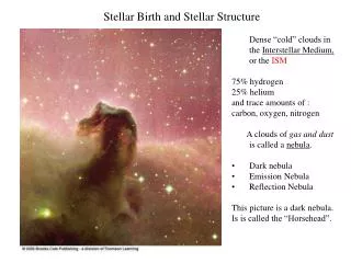
16. Life history of stars: Birth • Interstellar cloud of dust and cool gas: • Perturbed by external event: self-gravity starts contraction • If spinning, contraction leads to faster spin • High angular momentum material left behind in disc • Disc may form planets, and may also eject jets • Central blob radiates  initial isothermal collapse • When blob opaque, radiation trapped and temperature rises • Thermal pressure slows collapse • “Proto-star” – hot interior, cool exterior • Contraction releases just enough energy to balance radiation

17. Life history of stars: Energy sources • Gravitational energy, from contraction – if sole energy source for Sun (Kelvin, Helmholtz, 19th century), then timescale ~ E/L where E = gravitational energy of star, L = luminosity: • tKH = GM2/LR ~ 3107 yr for Sun. • But geology requires much longer timescale – only nuclear fuel provides this; nuclear binding energy releases up to ~1% of rest mass energy: EN ~ 0.01Mc2, so • tN ~ 0.01Mc2/L ~ 1.5 1011 yr for Sun. • Over-estimate, because not all mass of Sun is hot enough to be transformed. Strong mass dependence, because L  M4 – so, for 50 M,tN ~ 108 yr – massive stars were born recently.

18. Life history of stars: Life and death • Proto-star contracts until centre hot enough for hydrogen to fuse to helium • Nuclear energy source enough to balance radiation, and contraction ceases (no more need for gravitational energy) • Very little change for a nuclear timescale – i.e. until nuclear fuel exhausted • Series of phases of alternating contraction (releasing gravitational energy until centre hot enough) and further nuclear reactions (helium to carbon, etc, possibly up to iron) • After all possible nuclear fuels exhausted, star contracts to a dead compact object: white dwarf, neutron star or black hole.