Download
1 / 134
1.34k likes | 1.34k Vues
This paper explores the pioneers of water ecosystem modeling and the use of models for understanding the response of water bodies to eutrophication. It discusses the advantages of modeling and the steps involved in environmental modeling, including calibration and verification. The derivation of the basic transport equation is also discussed.

E N D
Biogeochemical Modeling with Focus on Eutrophication Process Ali Ertürk İstanbul University, Faculty of Aquatic Sciences erturkal@gmail.com
Pioneers of Water Ecosystem Modelling (1920’s) H.W. Streeter Earl B. Phelps
Pioneers of Water Ecosystem Modelling (1930’s) • Alfred J. Lotka • Vito Volterra Founders of Mathematical biology
Pioneers of Water Ecosystem Modelling(1940’s) • Raymond Lindeman (1915-1942*) *Yes he died so early being onne of the most brilliant minds in ecology
Pioneers of Water Ecosystem Modelling(1950’s) • G. G. Winberg • Eugene Odum
Pioneers of Water Ecosystem Modelling(1960’s) • Donald O’Connor • William Earl Dobbins
Pioneers of Water Ecosystem Modelling(1970’s) • Dominiq Ditoro • Robert V. Thomann
What is Model? A model is a “conceived image of reality”, or a theoretical construct, relating some stimulus to a response. Models are tools that are developed by using computer technology and they are used for determination of response of a water body to an effect depending on its physical, chemical, and biological characteristics. Models are used for idealization and simplification of real world systems to solve the problems.
Advantages of Modelling • Monitoring is expensive. Monitoring is an integral component of model development that provides necessary data for model validation. • However, monitoring campaigns are expensive and can usually not be supported financially for extended time spans. • On the other hand, validated models are less expensive to maintain and only need limited amounts of data (such as input data and forcings). Some of these data could be easily obtained from state agencies.
Advantages of Modelling • Models can spatially and temporally interpolate between measurement data points. It does not matter how dense a monitoring network is designed; it will never completely cover a study area in space and time. • Doubling the monitoring frequency also doubles the field study costs. However, models can estimate the variable values in any study area location at any time for which measurements are unavailable.
Advantages of Modelling • Modelling allows for the testing of several hypotheses and projects. Models can be used for "what if predictions" and to answer arising questions. • With models, scenarios can be tested before construction and the results can be analysed before spending large amounts of money. This advantage is extremely important for the investigating the optionsto rehabilitate an aquatic ecosystem
Advantages of Modelling • Predicting with monitoring only is nearly impossible. Even if monitoring is essential for model set-up, it will never predict future environmental parameters. • Prediction can only occur from numerical models that project state variable evolution into the future. Because this study is based on predicting the future, numerical modelling is used in this study.
Calibration Model calibration involves a comparison between simulation results and field measurements. Model calibration consists of changing values of model input parameters in an attempt to match field conditions within some acceptable criteria. This requires that field conditions at a site be properly characterized.
Verification • A statistically acceptable comparison between model results and a second (independent) set of field data for another year or at an alternate site; model parameters are fixed and no further adjustment is allowed after the calibration step. • Subsequent testing of a calibrated model to additional field data preferably under different external conditions to further examine model validity.
Growth of Biomass is More Complicated in Secondary Production Models
Definitions Basic dimensions Concentration [M] [L] [T] Mass Length Time Mass per unit volume [M∙L-3] Mass Flow Rate Flux Mass per unit time [M∙T-1] Mass flow rate through unit area [M∙L-2 ∙T-1]
The Transport Equation Mass balance for a control volume where the transport occurs only in one direction (say x-direction) Mass entering the control volume Mass leaving the control volume Dx Positive x direction
The Transport Equation The mass balance for this case can be written in the following form Equation 1
The Transport Equation A closer look to Equation 1 Flux [M∙L-2 ∙T-1] Flux [M∙L-2 ∙T-1] Concentration over time [M∙L-3 ∙T-1] Area [L2] Area [L2] Volume [L3] [L3]∙[M∙L-3∙T-1] = [M∙T-1] [L2]∙[M∙L-2∙T-1] = [M∙T-1] Mass over time Mass over time
The Transport Equation Change of mass in unit volume (divide all sides of Equation 1 by the volume) Equation 2 Rearrangements Equation 3
The Transport Equation The flux is changing in x direction with gradient of A.J1 A.J2 Dx Positive x direction Therefore Equation 4
The Transport Equation Equation 3 Equation 4 Equation 5
The Transport Equation Rearrangements Equation 5 Equation 6 Equation 7
Equation 7 The Transport Equation Rearrangements Finally, the most general transport equation in x direction is: Equation 8
The Transport Equation We are living in a 3 dimensional space, where the same rules for the general mass balance and transport are valid in all dimensions. Therefore x1 = x x2 = y x3 = z Equation 9 Equation 10
The Transport Equation • The transport equation is derived for a conservative tracer (material) • The control volume is constant as the time progresses • The flux (J) can be anything (flows, dispersion, etc.)
The advective flux can be analyzed with the simple conceptual model, which includes two control volumes. Advection occurs only towards one direction in a time interval.
Δx is defined as the distance, which a particle can pass in a time interval of Δt.The assumption is that the particles move on the direction of positive x only.
The number of particles (analogous to mass) moving from control volume I to control volume II in the time interval Δt can be calculated using the Equation below, where Equation 11 where Q is the number of particles (analogous to mass) passing from volume I to control volume IIin the time interval Δt[M], C is the concentration of any material dissolved in water in control volume I [M∙L-3], Δx is the distance [L] and A is the cross section area between the control volumes [L2].
Number of particles passing from I to II in Dt Division by time: Number of particles passing from I to II in unit time Division by cross-section area: Number of particles passing from I to II in unit time per unit area = FLUX Advective flux Equation 12
The Advective Flux Equation 12
The diffusive flux can be analyzed with the simple conceptual model too. This conceptual model also includes two control volumes. Diffusion occurs towards both directions in a time interval.
Δx is defined as the distance, which a particle can pass in a time interval of Δt. The assumption is that the particles move on positive and negative x directions. In this case there are two directions, which particles can move in the time interval of Δt.
Another assumption is that a particle does not change its direction during the time interval of Δt and that the probability to move to positive and negative x directions are equal (50%) for all particles. Therefore, there are two components of the diffusesivemass transfer, one from the control volume I to control volume II and the second from the control volume II to control volume I
50 % probability Equation 13 Equation 14 Equation 15 Equation 16