Download
1 / 18
180 likes | 501 Vues
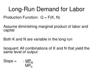
Long Run Demand for Labor. The long run. The long run is the time frame longer or just as long as it takes the firm to alter the physical plant or production facility. Thus the long run is that time period in which all inputs are variable. cost and output. K.

E N D
The long run • The long run is the time frame longer or just as long as it takes the firm to alter the physical plant or production facility. • Thus the long run is that time period in which all inputs are variable.
cost and output K On this slide I want to concentrate on one level of output, as summarized by the isoquant. Input combination E1, K1 could be used and have cost summarized by 4th highest isocost shown. E2, K2 would be cheaper, and E*, K* K1 K2 K* E E1 E2 E* is the lowest cost to produce the given level of output. Here the cheapest cost of the output occurs at a tangency point.
cost and output On the last screen we saw the tangency of an isoquant and isocost line shows the cheapest way to produce a certain level of output. The exception to reaching the tangency would be the short run when the amount of some input can not be changed to reach the tangency. In the long run all inputs can be changed in amount and thus the tangency point could be reached.
short run K Here the cheapest way to produce the output level as depicted in the isoquant would be to hire E*, K*. But maybe the firm has committed to having K1 units of capital. Thus the cost of this output is indicated by the fourth highest isocost line. K1 K2 K* E E1 E2 E* We could follow K1 out and see costs of other levels of output(by putting in more isoquants).
Tangency means equal slopes So in the long run when the firm has minimized cost we see a tangency of the slopes of the isoquant and an isocost line. The slope of the isocost line is the negative of the ratio of input prices -(w/r), And the slope of the isoquant is the negative of the ratio of marginal products -(MPE/ MPK). So the tangency means -(MPE/ MPK) = -(w/r) and the negative signs cancel out.
Economic meaning of this tangency The equality on the previous page can be rewritten as MPE/w = MPK/r. This says the ratio of the marginal product of each input to the inputs price has to be equal across all inputs for the firm to minimize the cost of making a level of output. Numerical example: Say MPE= 20, w = 10, MPK= 200, r = 100. Then we have 20/10 = 200/100 = 2/1. This means the last dollar spent on each input must yield the same increment to output. Here 2 units of output is obtained from the last dollar spent on each input.
Marginal product per dollar spent The statement on the end of the previous screen is that the marginal product per dollar spent must be equal across all inputs. What if it was not? Remember that if you take more of an input the marginal product diminishes (and thus if you take less the marginal product rises). Say the marginal product of capital is 100 and the price is 10 and the marginal product of labor is 20 and the price is 5. So per dollar spent you get 10 units of output from capital and 4 units from labor. Capital has more “bang for the buck,” so take more capital and less labor to move toward equality of ratios.
Another view We saw to have cost minimization we need MPE/w = MPK/r. If we take the inverse of these ratio’s we have w/MPE = r / MPK . Recall that that w is the wage and is the change in cost from hiring an additional laborer and MPE is the marginal product of labor, so the ratio is really the marginal cost of production. Another way to see the tangency condition is to say the marginal cost of output is the same for each input used.
profit maximization Firms want to maximize profit. To maximize profit they have to sell the right amount of output and produce that output at the lowest cost. We have just seen lowest cost means produce at a tangency point. In a competitive environment to maximize profit means to sell the output level where the price is equal to the marginal cost. Both of these statements imply w/MPE = r / MPK = p, and thus w = pMPE and r = pMPK. In other words, to maximize profit produce where the wage is equal to the value of the marginal product of labor and where the price of capital is equal to the value of the marginal product of capital.
wage fall and impact on isocost line K If the wage falls the isocost line rotates counterclockwise. The isocost line becomes flatter. More labor can be purchased given a cost amount. NOTE, the total cost or budgeted amount is the same on both lines. E
substitution and scale effects of a wage fall On the previous screen when the wage falls the budget flattens and shifts out and the firm moves from point P to point R. You can see the demand for labor by the firm rises as the wage falls. On the next slide this movement from P to R is broken into two moves: from P to Q and from Q to R. P to Q is called the substitution effect of a lower wage. Q to R is called the scale effect of a lower wage.
The substitution effect is a concept designed to show us the impact on the demand for labor when the wage changes, BUT the level of output is held constant. Note when the wage falls the firm takes more labor (and capital) and the level of output rises. To see the substitution effect in the graph, take the new isocost line and shift it in in a parallel fashion until you are back on the original isoquant. Thus output is back at its original level and we have the new wage. The movement from P to Q then is showing the change in the input mix because of the wage change, at the same level of output. As the wage falls, labor is relatively cheaper and thus firms take more of it in substitution of the relatively more expensive capital.
scale effect The movement from Q to R is called the scale effect. When the wage fell, the same amount of output can be made cheaper. But, for the same original cost, or budgeted amount, more output can be obtained. This is shown as the movement from Q to R. So, when the wage falls the scale effect says take more labor as the scale of output is increased.
A wage fall may mean that the profit maximizing level of output will have a higher cost than before. If so a lower wage may not only flatten an isoquant, but shift it out as well. The scale effect would be that much bigger. K R Q P E
Assignment 1 • In the notes we see the substitution and scale effects from a wage decline. • Show the same effects for a wage increase and give explanations of the logic of each effect.