Electric Potential

Electric Potential Chapter 25 Electric Potential Energy Electric Potential Equipotential Surfaces

For a collection of charges qi at positionsri the electric potential at r is the scalar sum: Electric Potential: the Bottom Line The electric potential V(r) is an easy way to calculate the electric field – easier than directly using Coulomb’s law. For a point charge at the origin: Calculate V and then find the electric field by taking the gradient:

Example: two point charges r a q q

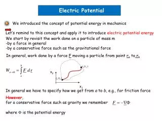
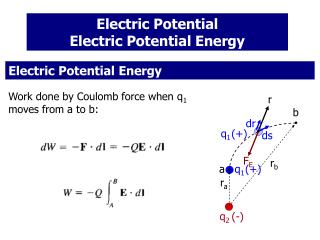
CONSERVATIVE FORCES A conservative force “gives back” work that has been done against it When the total work done by a force on an object moving around a closed loop is zero, then the force is conservative  F·dr = 0  F is conservative The circle on the integral sign indicates that the integral is taken over a closed path ° The work done by a conservative force, in moving and object between two points A and B, is independent of the path taken W=ABF·dris a function of A and B only – it is NOT a function of the path selected. We can define a potential energy difference as UAB=-W.

POTENTIAL ENERGY The change UAB in potential energy due to the electric force is thus UAB = -q ABE·dr UAB = UB – UA = potential energy difference between A and B Potential energy is defined at each point in space, but it is only the difference in potential energy that matters. Potential energy is measured with respect to a reference point (usually infinity). So we let A be the reference point (i.e, define UA to be zero), and use the above integral as the definition of U at point B.

L A B • • dl UAB =q E L POTENTIAL ENERGY IN A CONSTANT FIELD E E The potential energy difference between A and B equals the work necessary to move a charge +q from A to B UAB = UB – UA = -  q E·dl But E = constant, and E.dl = -E dl, so: UAB = -  q E · dl =  q E dl = q E  dl = q E L

ELECTRIC POTENTIAL DIFFERENCE The potential energy U depends on the charge being moved. To remove this dependence, we introduce the concept of the electric potential V. This is defined in terms of the difference V: VAB = UAB / q = - ABE · dl Electrical Potential = Potential Energy per Unit Charge = line integral of -E·dl VAB = Electric potential difference between the points A and B. Units are Volts (1V = 1 J/C), and so the electric potential is often called the voltage. A positive charge is pushed from regions of high potential to regions of low potential.

E L A B • • dL VAB = E L ELECTRIC POTENTIAL IN A CONSTANT FIELD E VAB = UAB / q The electrical potential difference between A and B equals the work per unit charge necessary to move a charge +q from A to B VAB = VB – VA = -  E·dl But E = constant, and E.dl = -1 E dl, so: VAB = -  E·dl =  E dl = E  dl = E L UAB =q E L

VAB = -  AB E · dl Cases in which the electric field E is not aligned with dl E A •  • B The electric potential difference does not depend on the integration path. So pick a simple path. One possibility is to integrate along the straight line AB. This is convenient in this case because the field E is constant, and the angle  between E and dl is constant. B E . dl = E dl cos   VAB = - E cos   dl = - E L cos  A

VAB = -  AB E · dl VAB = - E L cos  Cases in which the electric field E is not aligned with dl E d A C • •   L • B Another possibility is to choose a path that goes from A to C, and then from C to B VAB = VAC + VCB VAC = E d VCB = 0 (E  dL) Thus, VAB = E d but d = L cos  = - L cos 

A B E E VAB = E L VAx = E x x L L Equipotential Surfaces (lines) For a constant field E Similarly, at a distance x from plate A All the points along the dashed line at x, are at the same potential. The dashed line is an equipotential line

E L Equipotential Surfaces (lines) x It takes no work to move a charge at right angles to an electric field E dl   E•dl = 0  V = 0 If a surface(line) is perpendicular to the electric field, all the points in the surface (line) are at the same potential. Such surface (line) is called EQUIPOTENTIAL EQUIPOTENTIAL  ELECTRIC FIELD

Equipotential Surfaces We can make graphical representations of the electric potential in the same way as we have created for the electric field: Lines of constant E

Lines of constant V (perpendicular to E) Lines of constant E Equipotential Surfaces We can make graphical representations of the electric potential in the same way as we have created for the electric field:

Lines of constant V (perpendicular to E) Lines of constant E Equipotential Surfaces We can make graphical representations of the electric potential in the same way as we have created for the electric field: Equipotential plots are like contour maps of hills and valleys. A positive charge would be pushed from hills to valleys.

Equipotential Surfaces How do the equipotential surfaces look for: (a) A point charge? E + (b) An electric dipole? - + Equipotential plots are like contour maps of hills and valleys. A positive charge would be pushed from hills to valleys. Equipotential plots are like contour maps of hills and valleys.

Electric Potential of a Point Charge The Electric Potential b What is the electrical potential difference between two points (a and b) in the electric field produced by a point charge q. Point Charge q  a q

Electric Potential of a Point Charge The Electric Potential b c Choose a path a-c-b. DVab = DVac + DVcb DVab = 0 because on this path Place the point charge q at the origin. The electric field points radially outwards. a q DVbc =

b c F=qtE a q Electric Potential of a Point Charge The Electric Potential First find the work done by q’s field when qt is moved from a to b on the path a-c-b. W = W(a to c) + W(c to b) W(a to c) = 0 because on this path Place the point charge q at the origin. The electric field points radially outwards. W(c to b) = hence W

b c VAB = UAB / qt F=qtE a q VAB = k q [ 1/rb – 1/ra ] Electric Potential of a Point Charge The Electric Potential And since

b c F=qtE a q VAB = k q [ 1/rb – 1/ra ] V = k q / r Electric Potential of a Point Charge The Electric Potential From this it’s natural to choose the zero of electric potential to be when ra Letting a be the point at infinity, and dropping the subscript b, we get the electric potential: When the source charge is q, and the electric potential is evaluated at the point r. Remember: this is the electric potential with respect to infinity

Potential Due to a Group of Charges • For isolated point charges just add the potentials created by • each charge (superposition) • For a continuous distribution of charge …

 dqi Potential Produced by aContinuous Distribution of Charge In the case of a continuous distribution of charge we first divide the distribution up into small pieces, and then we sum the contribution, to the electric potential, from each piece:

VA =  dVA =  k dq / r vol vol Potential Produced by aContinuous Distribution of Charge In the case of a continuous distribution of charge we first divide the distribution up into small pieces, and then we sum the contribution, to the electric potential, from each piece: In the limit of very small pieces, the sum is an integral A  r dVA = k dq / r Remember: k=1/(40)  dq

P r z dw w R Example: a disk of charge dq = s2pwdw Suppose the disk has radius R and a charge per unit area s. Find the potential at a point P up the z axis (centered on the disk). Divide the object into small elements of charge and find the potential dV at P due to each bit. For a disk, a bit (differential of area) is a small ring of width dw and radius w.

Electric Potential