Download
1 / 74
830 likes | 1.19k Vues
Camera terminology. a camera is defined by an optical center c and an image plane image plane (or focal plane) is at distance f from the camera center f is called the focal length camera center = optical center principal axis = the line through camera center orthogonal to image plane

E N D
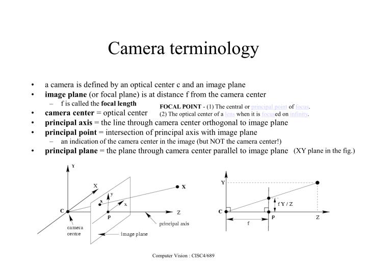
Camera terminology • a camera is defined by an optical center c and an image plane • image plane (or focal plane) is at distance f from the camera center • f is called the focal length • camera center = optical center • principal axis = the line through camera center orthogonal to image plane • principal point = intersection of principal axis with image plane • an indication of the camera center in the image (but NOT the camera center!) • principal plane = the plane through camera center parallel to image plane FOCAL POINT - (1) The central or principal point of focus. (2) The optical center of a lens when it is focused on infinity. (XY plane in the fig.) Computer Vision : CISC4/689
Pinhole Camera Terminology Image plane Optical axis Principal point/ image center Focal length Camera center/ pinhole Camera point Image point Computer Vision : CISC4/689
The equation of projection (Camera center) Computer Vision : CISC4/689
Cartesian coordinates: We have, by similar triangles, that (x, y, z) -> (f x/z, f y/z, -f) Ignore the third coordinate, and get The equation of projection Computer Vision : CISC4/689
Turn previous expression into HC’s HC’s for 3D point are (X,Y,Z,T) HC’s for point in image are (U,V,W) The camera matrix Computer Vision : CISC4/689
Issue camera may not be at the origin, looking down the z-axis extrinsic parameters freeing the origin from the camera center involves a translation C freeing the z-axis from the principal axis involves a rotation R one unit in camera coordinates may not be the same as one unit in world coordinates intrinsic parameters - focal length, principal point, aspect ratio, angle between axes, etc. Camera parameters Note the matrix dimensions Computer Vision : CISC4/689
Issues: what are intrinsic parameters of the camera? what is the camera matrix? (intrinsic+extrinsic) General strategy: view calibration object identify image points obtain camera matrix by minimizing error obtain intrinsic parameters from camera matrix Error minimization: Linear least squares easy problem numerically solution can be rather bad Minimize image distance more difficult numerical problem solution usually rather good, start with linear least squares Numerical scaling is an issue Camera calibration Computer Vision : CISC4/689
Homogeneous Coordinates • “Expanded” form is called homogeneous coordinates or projective space • Change to projective space by adding a scale factor (usually but not always 1): Computer Vision : CISC4/689
Homogeneous Coordinates: Projective Space • Equivalence is defined up to scale ¸ (non-zero for finite points) • Think of projective points in P2 as rays in R3, where z coordinate is scale factor • All Euclidean points along ray are “same” in this sense Computer Vision : CISC4/689
Leaving Projective Space • Can go back to non-homogeneous representation by dividing by scale factor and dropping extra coordinate: • This is the same as saying “Where does the ray intersect the plane defined by z = 1”? • Analogy to perspective projection, where f=1 (image plane) and lambda is z of any point in the ray. For different lambda’s along the line, projected point is the same, thus Equivalence class Computer Vision : CISC4/689
Ideal Points and Vanishing Points • Ideal points on the projective plane are located at infinity, and have coordinates of the form (x1,x2,0). There is just one free parameter in the coordinates of an ideal point because the scale of a homogeneous vector is arbitrary [x1(1,x2/x1,0)]- thus the set of all ideal points on the projective plane constitutes a line, called the ideal line. In the same way, the ideal points of projective 3-space have the form (x1,x2,x3,0). • The image of an ideal point under a projectivity is called a vanishing point, the image of an ideal line is called a vanishing line, and so on. An algebraic analysis of this configuration would describe the following: parallel lines meet at infinity at an ideal point; the image these lines meeting at the ideal point is at the vanishing point V (the image of the ideal point is V) - note that concurrency is preserved under a projective transformation, so concurrency at the ideal point in the world is reflected in concurrency at V in the image; Courtesy, CVonline Computer Vision : CISC4/689
Computer Vision : CISC4/689 Courtesy, CVonline
Figure:(a) One set of parallel lines on the plane is concurrent at the ideal point I1, and the other set is concurrent at I2 . The line through I1 and I2 is the ideal line (the horizon) of the plane. The image of I1 is the vanishing point V1, the image of I2 is the vanishing point V2, and the image of the ideal line is the vanishing line L. (b) Note that the plane formed by C and L has the same normal as the plane. Application: image stabilization! Project!!! (2005 paper) Computer Vision : CISC4/689 Courtesy, CVonline
Onto 3D • Coordinate systems • 3-D homogeneous transformations • Translation, scaling, rotation • Changes of coordinates • Rigid transformations Computer Vision : CISC4/689
Vector Projection • The projection of vector a onto u is that component of a in the direction of u Computer Vision : CISC4/689
Vector Cross Product • Definition: If a=(xa, ya, za)T and • b=(xb, yb, zb)T, then: c=aXb c is orthogonal to both aand b Computer Vision : CISC4/689 from Hill
Coordinate System: Definitions • Let x=(x, y, z)T be a point in 3-D space (R3). What do these values mean? • A coordinate system in Rn is defined by an origin o and n orthogonal basis vectors • In R3, positive direction of each axis X, Y, Z is indicated by unit vector i, j, k, respectively, where k=iXj(in a right-handed system) • Coordinate is length of projection of vector from origin to point onto axis basis vector—e.g., x= x . i o x Computer Vision : CISC4/689
3-D Camera Coordinates • Right-handed system • From point of view of camera looking out into scene: • +X right, {X left • +Y down, {Y up • +Zin front of camera, {Z behind Computer Vision : CISC4/689
Going from 2-D to 3-D • Points: Add z coordinate • Transformations: Become 4 x 4 matrices with extra row/column for z component—e.g., translation: Computer Vision : CISC4/689
3-D Scaling Computer Vision : CISC4/689
3-D Rotations • In 2-D, we are always rotating in the plane of the image, but in 3-D the axis of rotation itself is a variable • Three canonical rotation axes are the coordinate axes X, Y, Z • These are sometimes referred to • in aviation terms: (X)roll, (Y)pitch, and (Z)yaw, respectively from Hill Pitch is the angle that its longitudinal axis (running from tail to nose and along n) makes with horizontal plane. Courtesy: Wikepedia Computer Vision : CISC4/689 from Hill
3-D Euler Rotation Matrices • Similar to 2-D rotation matrices, but with coordinate corresponding to rotation axis held constant • E.g., a rotation about the X axis of µ radians: Computer Vision : CISC4/689
3-D Rotation Matrices • General form is: • Properties • RT= R-1 • Preserves vector lengths, angles between vectors • Upper-left block R3£3 is orthogonal matrix • Rows form orthonormal basis (as do columns): Length = 1, mutually orthogonal • So R3£3x projects point x onto unit vectors represented by rows of R3£3 Computer Vision : CISC4/689
Coordinate System Conversion • Camera coordinates C: Origin at center of camera, Z axis pointed in viewing direction • World coordinates W: Arbitrary origin, axes • Way to specify camera location, orientation (aka pose) in same frame as scene objects (we like to move camera to world, so as to convert world coordinates into camera coordinates) • Cx,Wx,: Same point in different coordinates Computer Vision : CISC4/689
Coordinate System Conversion • Camera coordinates C: Origin at center of camera, Z axis pointed in viewing direction • World coordinates W: Arbitrary origin, axes • Way to specify camera location, orientation (aka pose) in same frame as scene objects • Cx,Wx,: Same point in different coordinates Computer Vision : CISC4/689
Coordinate System Conversion • Camera coordinates C: Origin at center of camera, Z axis pointed in viewing direction • World coordinates W: Arbitrary origin, axes • Way to specify camera location, orientation (aka pose) in same frame as scene objects • Cx,Wx,: Same point in different coordinates Computer Vision : CISC4/689
Change of Coordinates: Special Case of Same Axes note: camera=calibration estimated. • Distinct origins, parallel basis vectors: If B is camera, Bx (camera) can be obtained by Ax (world) translated by its CG. Computer Vision : CISC4/689
Change of Coordinates: Special Case of Same Origin • Just need to rotate basis vectors so that they are aligned • Rotation matrix is projection of basis vectors in new frame Ex. World axes is (ia 0 0,0 ja 0,0 0 ka) and camera is (1 0 0, 0 1 0, 0 0 1) Check by multing (ia 0 0), etc. the rotation Matrix formed by world Axes. (ia 0 0).(ia 0 0) (0 ja 0).(0 ja 0) (0 0 ka).(0 0 ka) = [1 0 0], i.e, transformed to camera coords. (rotation of world in camera) Computer Vision : CISC4/689
3-D Rigid Transformations • Combination of rotation followed by translation without scaling • “Moves” an object from one 3-D position and orientation (pose) to another T R M Computer Vision : CISC4/689
3-D Transformations: Arbitrary Change of Coordinates • A rigid transformation can be used to represent a general change in the coordinate system that “expresses” a point’s location Computer Vision : CISC4/689
Rigid Transformations: Homogeneous Coordinates • Points in one coordinate system are transformed to the other as follows: • takes the camera to the world origin, transforming world coordinates to camera coordinates • If A is camera and B is world, inverse translation and inverse rotation Computer Vision : CISC4/689
Camera Projection Matrix • Using homogeneous coordinates, we can describe perspective projection as the result of multiplying by a 3 x 4 matrix P: (by the rule for converting between homogeneous and regular coordinates—this is perspective division) Computer Vision : CISC4/689
Camera Projection Matrix: Image Offsets Center of CCD matrix usually does not coincide with the principal point C0. This adds u0 and v0 to define in pixel units of C0 in retinal coordinate system. Computer Vision : CISC4/689
Factoring the Camera Matrix • Another way to write it: P=K ( Id 0 ) Camera calibration matrix Identity form of rigid transformation (with 4th row dropped) Computer Vision : CISC4/689
Camera Calibration Matrix • More general matrix allows: • Image coordinates with an offset origin (e.g., convention of upper left corner) • Non-square pixels = Different effective horizontal vs. vertical focal length • These four variables are known as the camera’s intrinsic parameters fu=f*su fv=f*sv Computer Vision : CISC4/689
Dealing with World Coordinates • Thus far we have assumed that points are in camera coordinates • Recall the definition of the world-to-camera coordinate rigid transformation: • In simpler form: And drop last row Computer Vision : CISC4/689
Combining Intrinsic & Extrinsic Parameters • The transformation performed by a pinhole camera on an arbitrary point in world coordinates can be written as: 3 x 4 projective camera matrix P has 10 degrees of freedom (DOF): 4 intrinsic, 3 rotation, 3 translation Computer Vision : CISC4/689
Skew ignored • The textbook has skew parameter included (pp. 29). • Since the camera coordinate system may also be skewed due to some manufacturing error, the angle between the two image axes is not equal (maybe close to 90 degrees). This adds up another unknown parameter • Easy to incorporate, just makes it 11 unknowns Computer Vision : CISC4/689
Applications • Estimates of the camera matrix parameters are critical in order to: • Know where the camera is and how it is moving • Deduce structural characteristics of the scene (i.e., 3-D information) • Place known objects (e.g., computer graphics) into a camera image correctly Computer Vision : CISC4/689
Camera Matrix • Linear systems of equations • Least-squares estimation • Application: Estimating the camera matrix Computer Vision : CISC4/689
Linear System • A general set of m simultaneous linear equations in n variables can be written as: Computer Vision : CISC4/689
Matrix Form of Linear System • This can be represented as a matrix-vector product: • Compactly, we write this as Ax = b Computer Vision : CISC4/689
Solving Linear Systems • If m=n (A is a square matrix), then we can obtain the solution by simple inversion: • If m>n, then the system is over-constrained and Ais not invertible • Use the pseudoinverse A+ =(ATA)-1AT to obtain least-squares solutionx= A+b (Ax=B, multiply both sides by A^t, etc.) Computer Vision : CISC4/689
Fitting Lines • A 2-D point x = (x, y) is on a line with slope m and intercept b if and only if y =mx + b • Equivalently, • So the line defined by two points x1, x2 is the solution to the following system of equations: Computer Vision : CISC4/689
Fitting Lines • With more than two points, there is no guarantee that they will all be on the same line • Least-squares solution obtained from pseudoinverse is line that is “closest” to all of the points Computer Vision : CISC4/689 courtesy of Vanderbilt U.
Example: Fitting a Line • Suppose we have points (2, 1), (5, 2), (7, 3), and (8, 3) • Then and x = A+b =(0.3571, 0.2857)T Computer Vision : CISC4/689
Example: Fitting a Line Computer Vision : CISC4/689
Homogeneous Systems of Equations • Suppose we want to solve Ax = 0 • There is a trivial solution x = 0, but we don’t want this. For what other values of x is Ax close to 0? • This is satisfied by computing the singular value decomposition (SVD) A = UDVT (a non-negative diagonal matrix between two orthogonal matrices) and taking x as the last column of V (unit singular vector) corresponding to the least eigenvalue. • Note that Matlab returns [U, D, V] = svd(A)-This is usually subject to constraints such as norm of x=1 Computer Vision : CISC4/689
Line-Fitting as a Homogeneous System • A 2-D homogeneous point x = (x, y, 1)T is on the line l = (a, b, c)T only when ax + by + c = 0 • We can write this equation with a dot product: x¢l = 0,and hence the following system is implied for multiple points x1, x2, ..., xn: Computer Vision : CISC4/689
Example: Homogeneous Line-Fitting • Again we have 4 points, but now in homogeneous form: (2, 1, 1), (5, 2, 1), (7, 3, 1), and (8, 3, 1) • Our system is: • Taking the SVD of A, we get: b=-1, a=.3571, c=0.2857..scaled differently C ompare tox =(0.3571, 0.2857)T Computer Vision : CISC4/689