Download
1 / 16
170 likes | 295 Vues
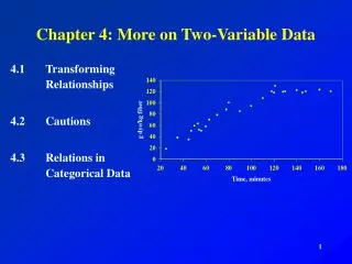
Chapter 4 More on Two-Variable Data. “Each of us is a statistical impossibility around which hover a million other lives that were never destined to be born†Loren Eiseley. 4.1 Some models for scatterplots with non-linear data (pp. 176-197). Exponential growth Growth or decay function Form:

E N D
Chapter 4More on Two-Variable Data “Each of us is a statistical impossibility around which hover a million other lives that were never destined to be born” Loren Eiseley
4.1Some models for scatterplots with non-linear data (pp. 176-197) • Exponential growth • Growth or decay function • Form: • Power function • Form:
Logarithms • Rules for logarithms
In other words… • The log of a product is the sum of the logs. • The log of a quotient is the difference of the logs. • The log of a power is the power times the log.
4.2Interpreting Correlation and Regression (pp. 206-214) Overview: • Correlation and regression need to be interpreted with CAUTION. Two variables may be strongly associated, but this DOES NOT MEAN that one causes the other. High Correlation does not imply causation! • We need to consider lurking variables and common response.
Extrapolation • The use of a regression line or curve to make a prediction outside of the domain of the values of your explanatory variable x that you used to obtain your line or curve. • These predictions cannot be trusted.
Lurking Variable • A variable that affects the relationship of the variables in the study. • NOT INCLUDED among the variables studied. • Example: strong positive association might exist between shirt size and intelligence for teenage boys. A lurking variable is AGE. • Shirt size and intelligence among teenage boys generally increases with age.
If there is a strong association between two variables x and y, any one of the following statements could be true: • x causes y: • Association DOES NOT imply causation, but causation could exist. • Both x and y are responding to changes in some unobserved variable or variables. • This is called common response. • The effect of x on y is hopelessly mixed up with the effects of other variables on y. • This is called confounding. • Always a potential problem in observational studies. • Can be somewhat controlled in experiments with a control group and a treatment group.
4.3Relations in Categorical Data (pp. 215-226) Overview: • We can see relations between two or more categorical variables by setting up tables. • So far, we have studied relationships with a quantitative response variable.
Notation • Prob(X) is the probability that X is true. • Prob(X/Y) is the probability that X is true, given that Y is true
Two-way Table • Describes the relationship between two categorical variables: • Row variable • Column variable • Row totals and column totals give MARGINAL DISTRIBUTIONS of the two variables separately. • DO NOT give any information about the relationships between the variables. • Can be used in the calculation of probabilities.
Example: 200 employees of a company are classified according to the Table below, where A, B, and C are mutually exclusive. Have A Have B Have C Totals Female 20 40 60 120 Male 30 10 40 80 Totals 50 50 100 200
Example: (con’t) • What is the probability that a randomly chosen person is female? • Prob(F) = 120/200 = 60% • What is the probability that a randomly chosen person has property A? • Prob(A) = 50/200 = 25% • If a randomly chosen person is female, what is the probability that she has property B? • Prob(B/F) = 40/50 = 80% • Note: equals Prob(B and F)/Prob(B)
Example: (con’t) • If a randomly chosen person has property C, what is the probability that the individual is male? • Prob(M/C) = 40/100 = 40% • Note: equals Prob(C and M)/Prob(M) • If a randomly chosen person has B or C, what is the probability that the person is male? • Prob(M/B or C) = 50/150 = 33.3%
Simpson’s Paradox • The reversal of the direction of a comparison or an association when data from several groups are combined to form a single group. • Lurking variables are categorical. • An extreme form of the fact that observed associations can be misleading when there are lurking variables.
First Half of BB Season Hits Times Bat at bat avg. Caldwell 60 200 .300 Wilson 29 100 .290 Second Half of BB Season Hits Times Bat at bat avg. 50 200 .250 1 5 .200 Example of Simpson’s Paradox Batting avgs. For entire season: Caldwell: 110/400 = .275 Wilson: 30/105 = .286 Calwell had a better avg. than Wilson in each half; however, Caldwell ends up with a LOWER OVERALL avg. than Wilson.