Hash Tables

1. Hash Tables CIS 606 Spring 2010

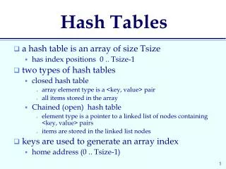
2. Hash tables • Many applications require a dynamic set that supports only the dictionary operations INSERT, SEARCH, and DELETE. Example: a symbol table in a compiler. • A hash table is effective for implementing a dictionary. • The expected time to search for an element in a hash table is O(1), under some reasonable assumptions. • Worst-case search time isΘ(n), however.

3. Hash tables • A hash table is a generalization of an ordinary array. • With an ordinary array, we store the element whose key is kin position kof the array. • Given a key k, we find the element whose key is k by just looking in the kth position of the array. This is called direct addressing. • Direct addressing is applicable when we can afford to allocate an array with one position for every possible key.

4. Hash tables • We use a hash table when we do not want to (or cannot) allocate an array with one position per possible key. • Use a hash table when the number of keys actually stored is small relative to the number of possible keys. • A hash table is an array, but it typically uses a size proportional to the number of keys to be stored (rather than the number of possible keys). • Given a key k, don’t just use k as the index into the array. • Instead, compute a function of k, and use that value to index into the array. We call this function a hash function.

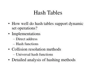
5. Hash tables • Issues that we’ll explore in hash tables: • How to compute hash functions. We’ll look at the multiplication and division methods. • What to do when the hash function maps multiple keys to the same table entry. We’ll look at chaining and open addressing.

6. Direct-address tables • Scenario • Maintain a dynamic set. • Each element has a key drawn from a universe U= {0; 1; . . .; m– 1} where misn’t too large. • No two elements have the same key. • Represent by a direct-address table, or array, T[0 . . . m– 1]: • Each slot, or position, corresponds to a key in U. • If there’s an element xwith key k, then T[k] contains a pointer to x. • Otherwise,T[k] is empty, represented by NIL.

7. Direct-address tables

8. Hash tables • The problem with direct addressing is if the universe U is large, storing a table of size |U| may be impractical or impossible. • Often, the set K of keys actually stored is small, compared to U, so that most of the space allocated for T is wasted. • When K is much smaller than U, a hash table requires much less space than a direct-address table. • Can reduce storage requirements to Θ(|K|). • Can still get O(1)search time, but in the average case, not the worst case.

9. Hash tables • Idea • Instead of storing an element with key kin slot k, use a function hand store the element in slot h(k). • We call ha hash function. • h: U➙ {0; 1; . . . ; m– 1}, so that h(k) is a legal slot number in T . • We say that khashes to sloth(k). • Collisions • When two or more keys hash to the same slot.

10. Collisions • Can happen when there are more possible keys than slots (|U| > m). • For a given set K of keys with |K| ≤ m, may or may not happen. Definitely happens if |K| > m. • Therefore, must be prepared to handle collisions in all cases. • Use two methods: chaining and open addressing. • Chaining is usually better than open addressing. We’ll examine both.

11. Collision resolution by chaining

12. Collision resolution by chaining • Insertion: • CHAINED-HASH-INSERT(T,x) insert xat the head of list T[h(key[x])] • Worst-case running time is O(1). • Assumes that the element being inserted isn’t already in the list. • It would take an additional search to check if it was already inserted. • Search: • CHAINED-HASH-SEARCH(T, k) search for an element with key kin list T[h(k)]. • Running time is proportional to the length of the list of elements in slot h(k). • Deletion: • CHAINED-HASH-DELETE(T, x) delete x from the listT[h(key[x])] • Given pointer xto the element to delete, so no search is needed to find this element. • Worst-case running time is O(1) time if the lists are doubly linked. • If the lists are singly linked, then deletion takes as long as searching, because we must find x’s predecessor in its list in order to correctly update next pointers.

13. Analysis of hashing with chaining • Given a key, how long does it take to find an element with that key, or to determine that there is no element with that key? • Analysis is in terms of the load factor α = n / m. • n= # of elements in the table. • m= # of slots in the table = # of (possibly empty) linked lists. • Load factor is average number of elements per linked list. • Can have α< 1,α> 1 or α= 1. • Worst case is when all n keys hash to the same slot ⇒ get a single list of length n ⇒ worst-case time to search isθ(n), plus time to compute hash function.! • Average case depends on how well the hash function distributes the keys among the slots.

14. Analysis of hashing with chaining • We focus on average-case performance of hashing with chaining. • Assume simple uniform hashing: any given element is equally likely to hash into any of the mslots. • For j = 0, 1, …, m– 1, denote the length of list T[j] by nj. Then n= n0 + n1 . + … + nm-1 . • Average value of njis E[nj] = α = n / m. • Assume that we can compute the hash function in O(1) time, so that the time required to search for the element with key kdepends on the lengthnh(k) of the list T[h(k)].

15. Analysis of hashing with chaining • We consider two cases: • If the hash table contains no element with key k, then the search is unsuccessful. • If the hash table does contain an element with key k, then the search is successful.

16. Unsuccessful search • Theorem • An unsuccessful search takes expected time θ(1 + α) • Proof • Simple uniform hashing ⇒ any key not already in the table is equally likely to hash to any of the mslots. • To search unsuccessfully for any key k, need to search to the end of the listT[h(k)]. This list has expected length E[nh(k)] = α. Therefore, the expected number of elements examined in an unsuccessful search is α. • Adding in the time to compute the hash function, the total time required is θ(1 + α).

17. Successful search • The expected time for a successful search is also θ(1 + α). • The circumstances are slightly different from an unsuccessful search. • The probability that each list is searched is proportional to the number of elements it contains. • Theorem • A successful search takes expected time θ(1 + α).

18. Successful search • Proof • (omitted)

19. Hash functions • What makes a good hash function? • Ideally, the hash function satisfies the assumption of simple uniform hashing. • In practice, it’s not possible to satisfy this assumption, since we don’t know in advance the probability distribution that keys are drawn from, and the keys may not be drawn independently. • Often use heuristics, based on the domain of the keys, to create a hash function that performs well.

20. Keys as natural numbers • Hash functions assume that the keys are natural numbers. • When they’re not, have to interpret them as natural numbers. • Example: Interpret a character string as an integer expressed in some radix notation. Suppose the string is CLRS: • ASCII values: C = 67, L = 76, R = 82, S = 83. • There are 128 basic ASCII values. • So interpret CLRS as (67*1283) + (76*1282) + (82*1281) + (83*1280)= 141,764,947.

21. Division method • h(k) = kmod m. • Example: m= 20 and k = 91 ⇒ h(k) = 11. • Advantage: Fast, since requires just one division operation. • Disadvantage: Have to avoid certain values of m: • Powers of 2 are bad. If m= 2p for integer p, thenh(k)is just the least significant pbits of k. • If kis a character string interpreted in radix2p(as in CLRS example), then m = 2p-1 is bad: permuting characters in a string does not change its hash value (Exercise 11.3-3). • Good choice for m: A prime not too close to an exact power of 2.

22. Multiplication method • Choose constant A in the range 0 < A < 1. • Multiply key kby A. • Extract the fractional part of kA. • Multiply the fractional part by m. • Take the floor of the result. • Disadvantage: Slower than division method. • Advantage: Value of mis not critical.

23. (Relatively) easy implementation: • Choose m= 2p for some integer p. • Let the word size of the machine be wbits. • Assume that kfits into a single word. (ktakes wbits.) • Let sbe an integer in the range 0 < s< 2w. (stakes wbits.) • Restrict A to be of the form s/2w.

24. (Relatively) easy implementation:

25. (Relatively) easy implementation: • Multiply kby s. • Since we’re multiplying two w-bit words, the result is 2w bits, r12w+r0, wherer1 is the high-order word of the product andr0 is the low-order word. • r1 holds the integer part of kA (bkAc) andr0 holds the fractional part of k A (k A mod 1 = k A – floor( k A)). Think of the “binary point” (analog of decimal point, but for binary representation) as being betweenr1 and r0 . Since we don’t care about the integer part of k A, we can forget aboutr1 and just user0 . • Since we want floor( m (k A mod 1)), we could get that value by shiftingr0 to the left by p= lgmbits and then taking the pbits that were shifted to the left of the binary point. • We don’t need to shift. The pbits that would have been shifted to the left of the binary point are the pmost significant bits ofr0 . So we can just take these bits after having formedr0 by multiplying kby s.

26. Example • m= 8 (implies p= 3), w= 5, k= 21. Must have 0 < s< 25; choose s= 13 ⇒ A = 13/32.

27. How to choose A: • The multiplication method works with any legal value of A. • But it works better with some values than with others, depending on the keys being hashed. • Knuth suggests using A ≈ (√5 – 1)/2.

28. Universal hashing • Suppose that a malicious adversary, who gets to choose the keys to be hashed, hasseen your hashing program and knows the hash function in advance. Then he could choose keys that all hash to the same slot, giving worst-case behavior. • One way to defeat the adversary is to use a different hash function each time. Youchoose one at random at the beginning of your program. Unless the adversary knows how you’ll be randomly choosing which hash function to use, he cannot intentionally defeat you. • Just because we choose a hash function randomly, that doesn’t mean it’s a good hash function. What we want is to randomly choose a single hash function from a set of good candidates.

29. Universal hashing • Consider a finite collection H of hash functions that map a universe U of keys into the range {0; 1; . . . ; m– 1}. H is universal if for each pair of keys k; l∈U, where k ≠ l, the number of hash functions h∈ H for which h(k) = h(l) is ≤ |H |/m. • Put another way,H is universal if, with a hash function hchosen randomly from H , the probability of a collision between two different keys is no more than than 1/m chance of just choosing two slots randomly and independently.

30. Universal hashing • Why are universal hash functions good? • They give good hashing behavior: • Theorem: Using chaining and universal hashing on key k: • If k is not in the table, the expected length E[nh(k)] of the list that khashes to is ≤ α. • If k is in the table, the expected length E[nh(k)] of the list that holds kis ≤ α + 1. • Corollary Using chaining and universal hashing, the expected time for each SEARCH operation is O(1). • They are easy to design.

31. Open addressing • An alternative to chaining for handling collisions. • Idea • Store all keys in the hash table itself. • Each slot contains either a key or NIL. • To search for key k: • Compute h(k) and examine sloth(k). Examining a slot is known as a probe. • If sloth(k)contains key k, the search is successful. If this slot contains NIL, the search is unsuccessful. • There’s a third possibility: sloth(k)contains a key that is not k. We compute the index of some other slot, based on kand on which probe (count from 0: 0th, 1st, 2nd, etc.) we’re on. • Keep probing until we either find key k(successful search) or we find a slot holding NIL (unsuccessful search).

32. Open addressing

33. Pseudocode for searching • HASH-SEARCH returns the index of a slot containing key k, or NIL if the search is unsuccessful.

34. Pseudocode for insertion • HASH-INSERT returns the number of the slot that gets key k, or it flags a “hash table overflow” error if there is no empty slot in which to put key k.

35. Deletion • Cannot just put NIL into the slot containing the key we want to delete. • Suppose we want to delete key kin slot j. • And suppose that sometime after inserting key k, we were inserting key k0, and during this insertion we had probed slot j(which contained key k). • And suppose we then deleted key kby storing NIL into slot j. • And then we search for keyk0. • During the search, we would probe slot j before probing the slot into whichkey k0was eventually stored. • Thus, the search would be unsuccessful, even though keyk0is in the table.

36. Deletion • Solution: Use a special value DELETED instead of NIL when marking a slot as empty during deletion. • Search should treat DELETED as though the slot holds a key that does not match the one being searched for. • Insertion should treat DELETED as though the slot were empty, so that it can be reused. • The disadvantage of using DELETED is that now search time is no longer dependent on the load factorα.

37. How to compute probe sequences • The ideal situation is uniform hashing: each key is equally likely to have any of the m! permutations of <0; 1; . . .; m-1> as its probe sequence. (This generalizes simple uniform hashing for a hash function that produces a whole probe sequence rather than just a single number.) • It’s hard to implement true uniform hashing, so we approximate it with techniques that at least guarantee that the probe sequence is a permutation of<0; 1; . . .; m-1>. • None of these techniques can produce all m! probe sequences. They will make use of auxiliary hash functions, which map U→ {0; 1; . . .; m-1}.

38. Linear probing • Given auxiliary hash function h’, the probe sequence starts at slot h’(k) and continues sequentially through the table, wrapping after slot m- 1 to slot 0. • Given key kand probe number i(0 ≤ i< m), h(k; I) = (h’(k) + i) mod m. • The initial probe determines the entire sequence ⇒ only mpossible sequences. • Linear probing suffers from primary clustering: long runs of occupied sequencesbuild up. And long runs tend to get longer, since an empty slot preceded by ifull slots gets filled next with probability (i+ 1)/m. Result is that the average search and insertion times increase.

39. Quadratic probing • As in linear probing, the probe sequence starts ath’(k). Unlike linear probing, it jumps around in the table according to a quadratic function of the probe number:h(k;i) = (h’(k) + c1i + c2i2) mod m, where c1; c2 ≠ 0 are constants. • Must constrainc1, c2, and min order to ensure that we get a full permutation of <0; 1; . . .; m-1>. (Problem 11-3 explores one way to implement quadratic probing.) • Can get secondary clustering: if two distinct keys have the same h’ value, then they have the same probe sequence.

40. Double hashing

41. Analysis of open-address hashing