Relaxation and Transport in Glass-Forming Liquids

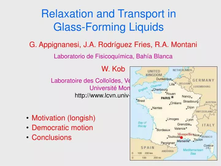
1. Relaxation and Transport in Glass-Forming Liquids G. Appignanesi, J.A. Rodríguez Fries, R.A. Montani Laboratorio de Fisicoquímica, Bahía Blanca W. Kob Laboratoire des Colloïdes, Verres et Nanomatériaux Université Montpellier 2 http://www.lcvn.univ-montp2.fr/kob • Motivation (longish) • Democratic motion • Conclusions

2. The problem of the glass-transition Angell-plot (Uhlmann) Strong increase of  with decreasing T Questions: • What is the mechanism for the slowing down? • What is the difference between strong and fragile systems? • What is the motion of the particles in this glassy regime? • ... • Most liquids crystallize if they are cooled below their melting temperature Tm • But some liquids stay in a (metastable) liquid phase even below Tm • one can study their properties in the supercooled state • Use the viscosity  to define a glass transition temp. Tg: (Tg) = 1013 Poise • make a reduced Arrhenius plot log() vs Tg/T

3. Model and details of the simulation Avoid crystallization binary mixture of Lennard-Jones particles; particles of type A (80%) and of type B (20%) parameters: AA= 1.0AB= 1.5BB= 0.5 AA= 1.0AB= 0.8BB= 0.85 • Simulation: • Integration of Newton’s equations of motion in NVE ensemble (velocity Verlet algorithm) • 150 – 8000 particles • in the following: use reduced units • length in AA • energy in AA • time in (m AA2/48 AA)1/2

4. Dynamics: The mean squared displacement • Mean squared displacement is defined as • r2(t)=|rk(t) - rk(0)|2 • short times: ballistic regime r2(t)  t2 • long times: diffusive regime r2(t)  t • intermediate times at low T: • cage effect • with decreasing T the dynamics slows down quickly since the length of the plateau increases • What is the nature of the motion of the particles when they start to become diffusive (=-process)?

5. Time dependent correlation functions • high T: after the microscopic • regime the correlation decays • exponentially • low T: existence of a plateau at • intermediate time (reason: cage effect); at long times the correlator • is not an exponential (can be fitted well by Kohlrausch-law) • Fs(q,t) = A exp( - (t/ )) • Why is the relaxation of the particles in the -process non-exponential? Possible explanation: Dynamical heterogeneities, i.e. there are “fast” and “slow” regions in the sample and thus the average relaxation is no longer an exponential • At every time there are equilibrium fluctuations in the density distribution; how do these fluctuations relax? • consider the incoherent intermediate scattering function Fs(q,t)Fs(q,t) = N-1(-q,t) (q,0) with (q,t) = exp(i qrk(t))

6. Dynamical heterogeneities: I • 2(t) is large in the caging regime • maximum of 2(t) increases with decreasing T  evidence for the presence of DH at low T • define t* as the time at which the maximum occurs • One possibility to characterize the dynamical heterogeneity (DH) of a system is the non-gaussian parameter • 2(t) = 3r4(t) / 5(r2(t))2 –1 • with the mean particle displacement r(t) ( = self part of the van Hove correlation function Gs(r,t) = 1/N i (r-|ri(t) – ri(0)|) )  • N.B.: For a gaussian process we have 2(t) = 0.

7. Dynamical heterogeneities: II • Define the “mobile particles” as the 5% particles that have the largest displacement at the time t* • Visual inspection shows that these particles are not distributed uniformly in the simulation box, but instead form clusters • Size of clusters increases with decreasing T

8. Dynamical heterogeneities: III • The mobile particles do not only form clusters, but their motion is also very cooperative: ARE THESE STRINGS THE -PROCESS? Similar result from simulations of polymers and experiments of colloids (Weeks et al.; Kegel et al.)

9. Existence of meta-basins T=0.5 • We see meta-basins (MB) • With decreasing T the residence time within one MB increases • NB: Need to use small systems (150 particles) in order to avoid that the MB are washed out • Define the “distance matrix” (Ohmine 1995) • 2(t’,t’’) = 1/N i|ri(t’) – ri(t’’)|2

10. ASD changes strongly when system leaves MB Dynamics: I • Look at the averaged squared displacement in a time  (ASD) of the particles in the same time window: • 2(t,) := 2(t- /2, t+ /2) • = 1/N i|ri(t+/2) – ri(t-/2)|2

11. Dynamics: II • Look at Gs(r,t’,t’+ ) = 1/N i(r-|ri(t’) – ri(t’+ )|)for times t’ that are inside a meta-basin • Gs(r,t’,t’+ ) is very similar to the mean curve ( = Gs(r, ) , the self part of the van Hove function)

12. Dynamics: III • Look at Gs(r,t’,t’+ ) = 1/N i(r-|ri(t’) – ri(t’+ )|)for times t’ that are at the end of a meta-basin, i.e. the system is crossing over to a new meta-basin • Gs(r,t’,t’+ ) is shifted to the right of the mean curve ( = Gs(r, ) ) • NB: This is not the signature of strings!

13. Fraction of mobile particles in the MB-MB transition is quite substantial ( 20-30 %) ! (cf. strings: 5%) • Strong correlation between m(t,) and 2(t,) Democracy • Define “mobile particles” as particles that move, within time , more than 0.3 • What is the fraction m(t,) of such • mobile particles?

14. Nature of the motion within a MB • Few particles move collectively; signature of strings (?)

15. Nature of the democratic motion in MB-MB transition • Many particles move collectively; no signature of strings

16. Summary • For this system the -relaxation process does not correspond to the fast dynamics of a few particles (string-like motion with amplitude O() ) but to a cooperative movement of 20-50 particles that form a compact cluster •  candidate for the cooperatively rearranging regions of Adam and Gibbs • Slowing down of the system is due to increasing cooperativity of the relaxing entities (clusters) • Qualitatively similar results for a small system embedded in a larger system • Reference: • PRL 96, 057801 (2006) (= cond-mat/0506577)