Download
1 / 30
300 likes | 316 Vues
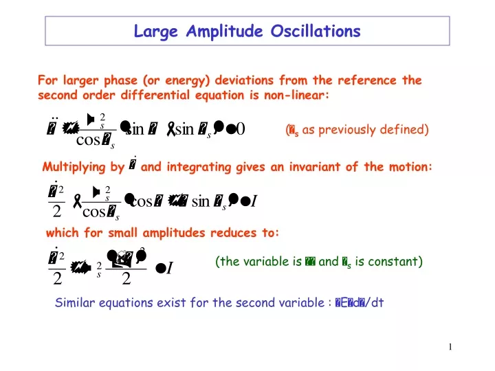
Large Amplitude Oscillations. For larger phase (or energy) deviations from the reference the second order differential equation is non-linear:. ( s as previously defined). Multiplying by and integrating gives an invariant of the motion:. which for small amplitudes reduces to:.

E N D
Large Amplitude Oscillations For larger phase (or energy) deviations from the reference the second order differential equation is non-linear: (s as previously defined) Multiplying by and integrating gives an invariant of the motion: which for small amplitudes reduces to: (the variable is and s is constant) Similar equations exist for the second variable : Ed/dt
Large Amplitude Oscillations (2) When reaches -s the force goes to zero and beyond it becomes non restoring. Hence -s is an extreme amplitude for a stable motion which in the phase space( ) is shown as closed trajectories. Equation of the separatrix: Second value m where the separatrix crosses the horizontal axis:
Energy Acceptance From the equation of motion it is seen that reaches an extremum when , hence corresponding to . Introducing this value into the equation of the separatrix gives: That translates into an acceptance in energy: This “RF acceptance” depends strongly on s and plays an important role for the electron capture at injection, and the stored beam lifetime.
RF Acceptance versus Synchronous Phase As the synchronous phase gets closer to 90º the area of stable motion (closed trajectories) gets smaller. These areas are often called “BUCKET”. The number of circulating buckets is equal to “h”. The phase extension of the bucket is maximum for s =180º (or 0°) which correspond to no acceleration . The RF acceptance increases with the RF voltage.
Potential Energy Function The longitudinal motion is produced by a force that can be derived from a scalar potential: The sum of the potential energy and kinetic energy is constant and by analogy represents the total energy of a non-dissipative system.
Ions in Circular Accelerators A =atomic number Q =charge state q = Q e Er = A E0 m = mr P = m v E = Er W = E – Er P = q B r E2 = p2c2 + Er2 Moreover: dr/r = 0 synchrotron dB/B = 0 cyclotron
From Synchrotron to Linac In the linac there is no bending magnets, hence there is no dispersion effects on the orbit and =0 and =1/2. cavity Ez s
From Synchrotron to Linac (2) In the linac there is no bending magnets, hence there is no dispersion effects on the orbit and =0 and =1/2. cavity Ez S or z
From Synchrotron to Linac (3) Since in the linac =0 and =1/2, the longitudinal frequency becomes: Moreover one has: leading to: Since in a linac the independant variable is z rather than t one gets:
Adiabatic Damping Though there are many physical processes that can damp the longitudinal oscillation amplitudes, one is directly generated by the acceleration process itself. It will happen in the synchrotron, even ultra-relativistic, when ramping the energy but not in the ultra-relativistic electron linac which does not show any oscillation. As a matter of fact, when Es varies with time, one needs to be more careful in combining the two first order energy-phase equations in one second order equation: The damping coefficient is proportional to the rate of energy variation and from the definition of s one has:
Adiabatic Damping (2) To integrate the previous equation, with variable coefficients, the method consists of choosing a solution similar to the one obtained without the damping term: Assuming time derivatives of parameters are small quantities (adiabatic limit), putting the solution in the equation and neglecting second order terms one gets: Integrating:
Adiabatic Damping (3) So far it was assumed that parameters related to the acceleration process were constant. Let’s consider now that they vary slowly with respect to the period of longitudinal oscillation (adiabaticity). For small amplitude oscillations the hamiltonian reduces to: with Under adiabatic conditions the Boltzman-Ehrenfest theorem states that the action integral remains constant: (W, are canonical variables) Since: the action integral becomes:
Adiabatic Damping (4) Previous integral over one period: leads to: From the quadratic form of the hamiltonian one gets the relation: Finally under adiabatic conditions the long term evolution of the oscillation amplitudes is shown to be:
Synchrotron Radiation Damping Light particles, such as electrons, radiate electro-magnetic energy when moving on circular orbits; that is typically the case in an electron synchrotron due to the bending magnetic field. Damping of longitudinal oscillations comes from the fact that the radiated power depends on the electron energy and on the magnetic field felt by the particle on its real trajectory: where is the classical electron radius. Note also that that the radiation leads to an energy lost per turn : automatically compensated by the RF system (synchronous particle).
Synchrotron Radiation Damping (2) Consider the energy deviation between a particle and the reference one: energy gain in the cavity dispersion effect Damping term: Focusing term:
Synchrotron Radiation Damping (3) The electron radiates on its orbit: The rate of variation of the energy loss with energy is then:
Synchrotron Radiation Damping (4) Since and considering the existence of a gradient the previous equation becomes: which often in the literature is expressed as: Leading to the damping constant:
Dynamics in the Vicinity of Transition Energy Introducing in the previous expressions: one gets:
Dynamics in the Vicinity of Transition Energy (2) t t In fact close to transition, adiabatic solution are not valid since parameters change too fast. A proper treatment would show that: will not go to zero E will not go to infinity t
Dynamics in the Vicinity of Transition Energy (3) Back to the general second order phase equation: Deriving the first term and looking for small phase deviations: Since: one gets:
Dynamics in the Vicinity of Transition Energy (4) Assuming: equivalent to: the resulting phase equation near transition becomes: with:
Dynamics in the Vicinity of Transition Energy (5) The previous equation has Bessel-Neumann type solutions symetric with respect to t: where A and B are initial conditions and: Expanding Bessel and Neumann function for small t leads to: Since energy deviation is proportional to the time derivative of phase deviation, deriving J and N and expanding one gets: showing that energy deviation does not go to infinity.
Stationary Bucket This is the case sins=0 (no acceleration) which means s=0 or . The equation of the separatrix for s= (above transition) becomes: Replacing the phase derivative by the canonical variable W: W Wbk and introducing the expression for s leads to the following equation for the separatrix: 0 2 with C=2Rs
Stationary Bucket (2) Setting = in the previous equation gives the height of the bucket: The area of the bucket is: Since: one gets:
Bunch Matching into a Stationary Bucket A particle trajectory inside the separatrix is described by the equation: s= W The points where the trajectory crosses the axis are symmetric with respect to s= Wbk Wb 0 2 m 2-m
Bunch Matching into a Stationary Bucket (2) Setting in the previous formulaallows to calculate the bunch height: or: This formula shows that for a given bunch energy spread the proper matching of a shorter bunch will require a bigger RF acceptance, hence a higher voltage ( short bunch means m close to ).
Effect of a Mismatch Starting with an injected bunch with short lenght and large energy spread, after a quarter of synchrotron period the bunch rotation shows a longer bunch with a smaller energy spread. W W For small oscillation amplitudes the equation of the ellipse reduces to: Ellipse area is called longitudinal emittance
Debunching Switching off the RF the stationary bucket vanishes and the bunch will debunch: W Φ W Φ