Download
1 / 20
200 likes | 299 Vues
A Simplified Dynamical System for Tropical Cyclone Intensity Evolution. Mark DeMaria, NESDIS/StAR Fort Collins, CO 80523 Presented at The 28 th AMS Conference on Hurricanes and Tropical Meteorology, April 28-May 2, 2008. Outline. The logistic growth equation model

E N D
A Simplified Dynamical System for Tropical Cyclone Intensity Evolution Mark DeMaria, NESDIS/StAR Fort Collins, CO 80523 Presented at The 28th AMS Conference on Hurricanes and Tropical Meteorology, April 28-May 2, 2008
Outline • The logistic growth equation model • Parameter estimation with the adjoint model • Applications • Simulation of individual storms • Real time intensity prediction • Evaluation of satellite retrievals • Pre-genesis prediction • Downscaling of climate simulations
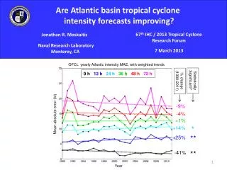
SHIFOR – 1988 Statistical SHIPS – 1991 Statistical-dynamical Operational 1995 GFDL – 1992 3-D dynamical Operational 1995 HWRF – 2007 3-D dynamical NHC Operational Intensity Models Model with Most Accurate 48 h Atlantic Intensity Forecasts
The Logistic Growth Equation dV/dt = V -(V/Vmpi)nV (A) (B) Term A: Growth term, related to shear, structure, etc Term B: Upper limit on growth as storm approaches its maximum potential intensity (Vmpi) LGE Parameters: (t) Growth rate Vmpi(t)MPI MPI relaxation rate n“Steepness” parameter
Analytic LGE Solutions for Constant and Vmpi Vs = Steady State V = Vmpi(/)1/n Let U = V/Vs and T = t dU/dT = U(1-Un) U(t) = Uo{enT/[1 + (enT-1)(Uo)n]}1/n 0 0
Parameter Estimation • Vmpi(t) from empirical formula as function of SST • (t) = a1S + a2C + a3SC + b • S(t) = Shear from NCEP/GFS model • C(t) = Convective instability from entraining plume model, input from GFS model soundings • Model determined by six constants • , n, a1, a2 , a3, b • LGE adjoint model provides method for estimating constants from fit to NHC best track • Intensity change over land from empirical inland wind decay model
Applications • Simulation of individual storms • Operational intensity forecasting • S-C Phase space and modified MPI diagrams • Evaluation of satellite soundings • Intensity forecasts starting before genesis • Down-scaling of climate models
Simulation of Individual Storms Use adjoint technique to find 6 LGEM constants Minimize error of single model forecast of entire storm lifecycle Use observed track, SST, S and C Examples Frances 2004: 15 day LGEM run Rita 2005: 8 day LGEM run
Tropical Depression • Tropical Storm • Non-major Hurricane • Major Hurricane Rita and Frances TracksIncluded in LGEM Simulations
Operational Intensity Forecasting • Single set of coefficients for all forecasts • Earlier version of LGEM run in real time at NHC with SHIPS model since 2006 • Multiple regression estimation of with SHIPS predictors • LGEM-MR • Separate regressions at each forecast time
6-Coefficient LGEM Forecast Applications • Time independent coefficients • Forecast can be of any length • Vastly reduced predictor set • SHIPS 420 coefficients • LGEM-MR 294 coefficients • LGEM 6 coefficients • Adjoint technique allows assimilation of complete storm history up to forecast time • SHIPS/LGEM-MR use past 12 hr • LGEM, LGEM-MR, SHIPS to be compared with 2008 sample
Fit of 6-Coefficient LGEM to Large Data Sample • Single set of 6 coefficients to fit 2001-2006 Atlantic forecasts • Defines (S,C)
Storm Properties Determined by Evolution in S-C plane Claudette 2003 Katrina 2005
Application of Steady State Solution Vs = Steady State = Vmpi(/)1/n n = 2.6 -1 = 39 hr = f(S,C) Vs is MPI modified by shear and convective instability
Other Applications • Ensemble intensity forecasting • Fast run time allows very large ensembles • Satellite retrieval evaluation • Calculate S, C, SST from retrievals and compare forecasts to runs with GFS input • Genesis/Intensity forecasts • Use NCEP “tracker” to identify genesis in GFS forecast, apply LGEM along model track • Climate model applications • Apply LGEM to “downscale” climate runs • Similar to use of CHIPS in Emanuel (2008)
Conclusions • The logistic growth equation model (LGEM) can be applied to tropical cyclone intensity evolution • LGEM and its adjoint provide a model with a vastly reduced predictor set • 6 vs. 420 for SHIPS model • The intensity evolution of most individual storms can be accurately simulated with SST, S and C input • LGEM with a multiple regression technique was more accurate that SHIPS in 2006-2007 real time forecasts • 6-coefficient version of LGEM has many potential applications