Download
1 / 53
530 likes | 687 Vues
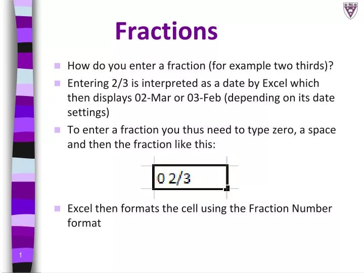
Fractions. How do you enter a fraction (for example two thirds)? Entering 2/3 is interpreted as a date by Excel which then displays 02-Mar or 03-Feb (depending on its date settings) To enter a fraction you thus need to type zero, a space and then the fraction like this:

E N D
Fractions • How do you enter a fraction (for example two thirds)? • Entering 2/3 is interpreted as a date by Excel which then displays 02-Mar or 03-Feb (depending on its date settings) • To enter a fraction you thus need to type zero, a space and then the fraction like this: • Excel then formats the cell using the Fraction Number format
Data Validation (1) • Data validation lets you define restrictions on what data can or should be entered in a cell. • You can configure data validation to prevent users from entering data that is not valid. • Can also • allow users to enter invalid data but warn them when they try to type it in the cell • provide instructions to help users know what to data to enter or correct errors
Data Validation (2) • To set up a cell or a range of cells so that it only accepts certain kinds of data: • Select the cells • Choose Data Validation from the Data Tools group on the Data tab of the Ribbon • Using the Data Validation dialog box will allow you to configure settings, messages and error messages
Data Validation (3) • EXAMPLE (slide 1/5):
Data Validation (4) • EXAMPLE (slide 2/5):
Data Validation (5) • EXAMPLE (slide 3/5):
Data Validation (6) • EXAMPLE (slide 4/5):
Data Validation (7) • EXAMPLE (slide 5/5):
Section 2 – Appearance and Formatting • The world is an unfortunately shallow place! • Appearance can be customised for ease of comprehension, clarity, impact • General rule of business: the higher up the corporate hierarchy a document is destined, the greater the effort that must be invested in formatting it • Sloppy formatting sends the message that the document or task is meaningless to the author, or that the author is uneducated
Formatting Data Formatting can be accomplished by selecting the cells/range of cells you want to format and • using the limited formatting options available from the Mini toolbar • right-clicking, and selecting Format Cells from the context menu, or • selecting the appropriate option from the Home tab (bigger picture soon!)
Formatting Data - Number If you choose to right-click you will be presented with the Format Cells dialog box. This has various tabs along the top, each of which allows the formatting of different things.
Formatting options on the Home tab (1) Increase/DecreaseFont Size Font Face Align Bottom Align Top Font Size Align Middle Orientation Bold Merge and Centre Align Left Italics Cell borders Align Right Font Colour Underscore Center Fill Colour Increase/Decrease Indent
Formatting options on the Home tab (2) Comma Style Conditional Formatting Format as Table Pre-defined Cell Styles Percent Increase/Decrease Decimal Currency
Conditional Formatting • Conditional Formatting allows you to format a cell according to its contents • E.g. If a product needed to make a 10% profit to be economically viable to produce, all cells below this threshold could be formatted to appear red/bold/etc
Using Styles (1) • A style is a combination of formatting characteristics such as alignment, font, border, or pattern • Applying a style applies this combination of formatting characteristics in one go
Using Styles (2) • To apply a style select the area to be formatted (Ctrl A to select an entire worksheet) and then Style from the drop-down menu on the Styles group of the Home tab of the Ribbon • Select your chosen style
Using Styles (3) • Excel has predefined styles or you can define your own • To define a style: • Choose New Cell Style from the drop-down menu on the Styles group of the Home tab of the Ribbon • In the Style dialog box name your style and set any options you want (including formatting) • OR • first format at least one cell with all the formatting characteristics you want for the style and then define as above
Painting Formats • Format painting allows you to take the formats set for a particular cell and copy them to other cells without using Styles or copying the data in the cell • To paint a format • select the cell that has the format you want to copy • Click the Format Painter button on the Clipboard section of the Home tab on the Ribbon • Select the cell/range of cells that you would like to format in the same manner
Inserting Illustrations (1) • 4 types of graphic can be inserted into a spreadsheet, namely Pictures (from files stored on your computer), Clip Art (pictures supplied with MS Office 2007), Shapes, and Smart Art diagrams (e.g. graphical lists, Venn diagrams and organisational charts) • To insert a graphic simply select the type of graphic you want from the Illustrations group of the Insert tab on the Ribbon
Inserting Illustrations (2) • If you have a picture saved somewhere that you wish to use, select Picture, browse to the location of your picture and select the file name • Alternatively select Clip Art
Inserting Illustrations (3) • Clip Art allows you to search for a suitable picture in the Clip Art Gallery • Once you spot a suitable picture, click on it to select it and it will be placed on your spreadsheet
Working with Illustrations • You can click and drag to move the image around • Clicking and dragging a sizing handle on one of the corners will resize the image • Further customisations can be achieved by double-clicking on the image - this brings up the thePicture Tools Formatting Gallery on the Ribbon (note the options)
Section 3 – Organising Data Sorting and Filtering • Not just for the compulsively neat! • Sorting rearranges data whereas filtering determines what data is visible at a given time • Sorting gives database-style functionality to spreadsheets allowing the user to prioritize certain data e.g. • Categories • Numerical data meeting certain criteria • Etc • Available from the Sort & Filter group of the Data tab on the Ribbon
Sorting (1) • To sort one simple column of data in ascending (A-Z) or descending (Z-A) order, select the data you want sorted (not including the column heading) and click on the Sort Ascending ( ) or Sort Descending ( ) buttons on the toolbar. • Excel is smart enough to recognise that certain types of formatting (like bolding) are likely to represent column headings and avoid sorting the heading into the data. Relying on this is risky...
Sorting (2) • If you use Sort Ascending or Sort Descending on multiple columns of data Excel will sort by the data in the first column only – why? Why shouldn’t you select each column separately and sort it? • If you use Sort Ascending or Sort Descending without selecting data first, Excel will attempt to make a smart selection as to the data you want sorted
Sorting (3) • To sort multiple columns of data in ascending (A-Z) or descending (Z-A) order without destroying the relationships between the data elements, select the data you want sorted and select Sort from the Data tab on the Ribbon.
Sorting (4) • Select which columns to sort by, the sort criteria, and in which order to sort • You can sort by more than one column by using the Add Level button
Filtering (1) • Filtering temporarily hides rows that do not meet specified criteria • The Filter button performs an automatic filter that displays a subset of data that meets certain criteria • Select data Data tab Sort & Filter group Filter
Filtering (2) • AutoFilter arrows appear on the lower right-hand corner of the column heading cells • Clicking the arrows displays a drop-down list of filtering options as well as the values appearing in the column • Select a filtering option or a value (to display only rows containing that value)
Moving Data • To copy or move data from one place to another you first need to select it. • Then use the cut/copy/paste options, accessed from the Clipboard group of the Home tab on the Ribbon
Paste Special • Paste offers a number of options such as Paste Special. • Paste Special offers a range of ways to paste things. • E.g. : If your spreadsheet uses a lot of Formulas, if you paste these into a blank spreadsheet the Formulas will then refer to blank empty cells and you’ll just see a series of zeroes. Using Paste Special you can choose to paste the values (totals, percentages etc) that were produced by the Formulas rather than the Formulas themselves to ensure that the data remains meaningful in its new location.
Paste Special • The Transpose option allows you to change the orientation of data you are pasting