Download
1 / 72
800 likes | 1.1k Vues
Image Segmentation. Chapter 10 Murat Kurt. 1 .1 Point, Line and Edge Detection. To detect a given property of an object we look at the intensity discontinuities. For this purpose we run a mask throughout the image. For a 3 × 3 mask, this procedure involves computing the quantity

E N D
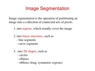
Image Segmentation Chapter 10 Murat Kurt
1.1 Point, Line and Edge Detection • To detect a given property of an object we look at the intensity discontinuities. • For this purpose we run a mask throughout the image. • For a 3×3 mask, this procedure involves computing the quantity and comparing it with a threshold value (zi is the intensity of the pixel associated with mask coefficientwi).
1.1 Point Detection • Using the mask shown in Figure 10.1, we say that an isolated point has been detected at the location on which the mask is centered if
1.1 Point Detection (cont.) • Point detection is implemented in MATLAB using function imfilterwith the mask above. >> w = [-1 -1 -1; -1 8 -1; -1 -1 -1]; >> f=imread('Fig1002(a)(test_pattern_with_single_pixel).tif'); >> g=abs(imfilter(double(f),w)); >> imshow(g) >> T=max(g(:)); >> g=g>=T; >> imshow(g)
1.2 Line Detection • Consider the following masks • If the first mask is moved around an image, it would respond more strongly to lines oriented horizontally. • With a constant background, the maximum response would result when the line passed through the middle of the mask. • Similarly the second, the third and the fourth mask ....
1.2 Line Detection (cont.) • Let R1 , R2 , R3 , and R4 denote the responses of masks in Figure 10.3. • If a point in the image | Ri | > |Rj |for all j ≠ i that point is said to be more likely associated with a line in the direction of mask i.
1.2 Line Detection (cont.) EXAMPLE 10.2: Detection of lines in a specified direction. >> w = [2 -1 -1; -1 2 -1; -1 -1 2]; >> g=imfilter(double(f),w); >> imshow(g, []) %Fig. 10.4(b) >> gtop = g(1:120, 1:120); >> gtop = pixeldup(gtop, 4); >> figure, imshow(gtop, []) %Fig. 10.4(c) >> gbot = g(end-119:end, end-119:end); >> gbot = pixeldup(gbot, 4); >> figure, imshow(gbot, []) %Fig. 10.4(d) >> g = abs(g); >> figure, imshow(g, []) %Fig. 10.4(e) >> T = max(g(:)); >> g = g >= T; >> figure, imshow(g) %Fig. 10.4(f)
1.3 Edge Detection • Edge detection is a most common approach for detecting meaningful discontinuties in intensity values. • Such discontinuties are detected by using first and second order derivatives. • The first order derivative of choice in image processing is the gradient which is defined as the vector.
1.3 Edge Detection (cont.) • A fundemental property of the gradient vector is that it points in the direction of the maximum rate of change of f at coordinates (x, y). The angle at which maximum rate of change occurs is
1.3 Edge Detection (cont.) • The second-orderderivatives in image processing are generally computed using the Laplacian. That is, the Laplacian of a 2-D function f(x, y) is formed from second-order derivatives, as follows: • The Laplacian is seldom used by itself for edge detection because, as a second-order derivative, it is unacceptably sensitive to noise, its magnitude produces double edges, and it is unable to detect edge direction. However, the Laplacian can be powerful complement when used in combination with other edge-detection techniques. For example, although its double edges make it unsuitable for edge detection directly, this property can be used for edge location.
1.3 Edge Detection (cont.) • The basic idea behind the edge detection is to find places in an image where the intensity changes rapidly using one of the two general criteria: • Find places where the first derivative of the intensity is greater in the magnitude than a specified threshold. • Find places where the second derivative of the intensity has a zero crossing. • The IPT function edge provides several derivative estimators based on the above criteria. [g,t]=edge[f, 'method ', parameters)
1.3 Edge Detection (cont.) Sobel Edge Detector: • This detector uses the masks in Fig. 10.5(b) to approximate digitally the first derivatives Gx and Gy. • The gradient at the center point in a neighborhood is computed as follows: • Then we say that a pixel at location (x, y) is an edge pixel if g≥T at that location.
1.3 Edge Detection (cont.) The calling syntax for the Sobel detectoris [g,t]=edge(f, 'sobel', T,dir) where dir specifies the preferred direction of the edges detected:'horizontal ', ' vertical ', ' both '
1.3 Edge Detection (cont.) a b c d
1.3 Edge Detection (cont.) Prewitt Edge Detector: • This detector usess the masks in Fig. 10.5(c) to approximate digitally the first derivatives Gx and Gy. • The calling syntax for the Prewitt edge detectoris [g,t]=edge(f, ‘prewitt', T,dir)
1.3 Edge Detection (cont.) Robert Edge Detector: • This detector usess the masks in Fig. 10.5(d) to approximate digitally the first derivatives Gx and Gx. • The calling syntax for the Robert edge detectoris [g,t]=edge(f, ‘roberts', T,dir) • This detector is used considerably less than the others in Fig. 10.5 due in part to its limited functionality (e.g., it is not symmetric and cannot be generalized to detect edges that are multiples of 45°). • However, it still is used frequently in hardware implementations where simplicity and speed are dominant factors.
1.3 Edge Detection (cont.) Laplacian of a Gaussian(LoG) Detector: • Consider the Gaussian function where and is the variance. • An image is blured if this smoothing function is convolved with it. The degree of bluring is determined by the value of . • The Laplacian (the second derivative with respect to r) of this function is
1.3 Edge Detection (cont.) Laplacian of a Gaussian(LoG) Detector: • Filtering (convolving) an image with is the same as filtering the image with the smoothing function first and then computing the Laplacian of the result. • This is the key concept underlying the LoG detector. • We convolve the image with knowing that it has two effects • It smoothes the image (thus reducing noise) • It computes the Laplacian which yields a double-edge image. • Locating edges then consists of finding zero crossing between the double edges.
1.3 Edge Detection (cont.) The calling syntax for the LoG detectoris [g,t]=edge(f, ‘log', T, sigma)
1.3 Edge Detection (cont.) Canny Edge Detector: • This detector is the most powerful edge detector provided by function edge. The method can be summarized as follows: • The image is smoothed using a Gaussian filter with a specified standard deviation σ. • The local gradient and edge direction are computed at each point. An edge point is defined to be a point whose strength is locally maximum in the direction of the gradient.
1.3 Edge Detection (cont.) Canny Edge Detector: • The edge points give rise to ridges in the gradient magnitude image. The algorithm then tracks along the top of these ridges and sets to zero all pixels that are not actually on the ridge top so as to give a thin line in the output.The ridge pixels are then thresholded using two thresholds T1 and T2 with T1<T2. Ridge pixels with values greather than T2 are said to be strong edge pixels Ridge pixels with values between T1 and T2 are said to be weak edge pixels. • Finally the algorithm performsedge linking by incorporating the weakpixels that are 8-connected to the strong pixels
1.3 Edge Detection (cont.) The calling syntax for the Canny edge detectoris [g,t]=edge(f, ‘canny', T, sigma) where T is a vector T =[T1, T2], containing the two thresholds explained in step 3 of the preceding procedure, and sigma is the standard deviation of the smoothing filter.
1.3 Edge Detection (cont.) EXAMPLE 10.3: Edge extraction with the Sobel detector. >> [gv, t] = edge(f, ‘sobel’, ‘vertical’); >> imshow(gv) %Fig. 10.6(b) >> gv = edge(f, ‘sobel’, 0.15, ‘vertical’) >> imshow(gv) %Fig. 10.6(c) >> gboth = edge(f, ‘sobel’, 0.15) >> imshow(gboth) %Fig. 10.6(d) >> w45 = [-2 -1 0; -1 0 1; 0 1 2]; >> g45 = imfilter(double(f), w45, ‘replicate’); >> T = 0.3*max(abs(g45(:)));g45 = g45 >= T; >> figure, imshow(g45); %Fig. 10.6(e) >> wm45 = [-2 -1 0; -1 0 1; 0 1 2]; >> gm45 = imfilter(double(f), wm45, ‘replicate’); >> T = 0.3*max(abs(gm45(:)));gm45 = gm45 >= T; >> figure, imshow(gm45); %Fig. 10.6(f)
1.3 Edge Detection (cont.) Example:
1.3 Edge Detection (cont.) EXAMPLE 10.4: Comparision of the Sobel, LoG, and Canny edge detectors. >> [g_sobel_default, ts] = edge(f, ‘sobel’); %Fig. 10.7(a) >> [g_log_default, tlog] = edge(f, ‘log’); %Fig. 10.7(c) >> [g_canny_default, tc] = edge(f, ‘canny’); %Fig. 10.7(e) >> g_sobel_best = edge(f, ‘sobel’, 0.05); %Fig. 10.7(b) >> g_log_best = edge(f, ‘log’, 0.03, 2.25); %Fig. 10.7(d) >> g_canny_best = edge(f, ‘canny’, [0.04 0.10], 1.5); %Fig. 10.7(f)
1.3 Edge Detection (cont.) Example:
2 Thresholding • Thresholding enjoys a central position in image segmentation. • Suppose that the following intensity histogram corresponds to an image , composed of light objects on a dark background in such a way that object and background pixels have intensity levels grouped into two dominant modes. • Any point for which f(x,y)≥T is called an object point otherwise is called a background point.
2 Thresholding (cont.) • In other words, the thresholded image g(x,y) is defined as • When T is a constant, this approach is called global thresholding.
2.1 Global Thresholding • One way to choose a threshold is by visual inspection of the image histogram. • Another method of choosing T is by trial and error. • For choosing threshold automatically: • Select an initial estimate of T. (A suggested initial estimate is the midpoint between the minimum and maximum intensity values in the image.) • Segment the image usingT. This will produce two groups of pixels G1 and G2 . • Compute the average intensity values μ1 and μ2.for pixel in G1 and G2 . • Compute a new threshold value: • Repeat steps 2-4 until the diference in T in successive iteration is smaller than a predifined parameter T0.
2.1 Global Thresholding (cont.) The Otsu Method • We start by treating the normalized histogram as a discrete pdf with where n is the number of pixels in the image, nq is the number of pixels that have intensity level rq and L is the total number of possible intensity levels in the image. • Suppose that a threshold k is chosen s.t. C0 is the set of pixels with levels [0, 1, ..., k-1] and C1 is the set of pixels with levels [k, k+1, ..., L-1]. • Otsu method choses the threshold value k that maximizes the between-class variance
2.1 Global Thresholding (cont.) The Otsu Method Otsu method choses the threshold value k that maximizes the between-class variance where
2.1 Global Thresholding (cont.) The following function takes an image, computes its histogram, and then finds the threshold value that maximizes the between-class variance. The threshold is returned as a normalized value between 0.0 and 1.0, T=graythresh(f) where f is the input image and T is the resulting threshold.
2.1 Global Thresholding (cont.) EXAMPLE 10.7: Computing global thresholds. >> T = 0.5*(double(min(f(:))) + double(max(f(:)))); >> done = false; >> while ~done g = f >= T; Tnext = 0.5*(mean(f(g)) + mean(f(~g))); done = abs(T - Tnext) < 0.5;T = Tnext; end >> T T = 101.47 >> T2 = graythresh(f) %Fig. 10.13(b) shows the image thresholded using T2 T2 = T2 * 255 101
2.2 Local Thresholding Global thresholding methods can fail when the background illumination is un-even as illustrated in Figs 9.26(a) and (b)
2.2 Local Thresholding (cont.) • A common practice in such situations is to preprocess the image to compansate for the illumination problems and then apply a global threshold to the preprocessed image. • The improved thresholding resul is shown in Fig. 9.26(e) was computed by applying a morphological top-hat operation and then using graytrthresh on the result. • We can show that this process is equivalent to thresholding f(x, y) with a locally varying threshold function T(x,y): where • The image is the morphological opening of f , and the constant is the result of function graythresh applied to .
3. Region-Based Segmentation • The objective of segmentation is to partition an image into regions. In Sections 10.1 and 10.2, we approached this problem by finding boundaries between regions based on discontinuities in intensity levels, whereas in Section 10.3 segmentation was accomplished via thresholds based on the distribution of pixel properties, such as intensity values. • In this section we discuss segmentation techniques that are based on finding the regions directly.
3.1 Basic formulation • Let R represent the entire image region. • We may view segmentation as a process that partitions R into subregions R1, R2, ..., Rn, such that • Ri (i=1,2, ...,n)is a connected region. • Ri ∩ Rj =Øfor all i and j, i≠j. • P(Ri)=TRUEfor i=1,2, ...,n • P(Ri U Rj)=FALSEfor any adjacent regions Ri and Rj
3.2 Region Growing • Region growing is a procedure that groups pixels or subregions into larger regions based on predefined criteria for growth. • The basic approach is to start with a set of seed points and from these grow regions by appending to each seed those neighbouring pixels that have predefined properties similar to the seed. • The selection of similarity criteria depends not only on the problem under consideration but also on the type of image data available.
3.2 Region Growing(cont.) Problems associated with region growing: • Descriptors alone can yield misleading results if connectivityis not used in the region-growing process. • Stopping rule: Basically growing a region should stop when no more pixels satisfy the criteria for inclusion in that region. Criteria such as texture and color are local and do not take into account the history of region growth. Additional criteria that increase the power of a region-growing algorithm utilize the concept of size, likeness between a candidate pixel and the pixels grown so far (such as a comparison of the intensity of a candidate and the average intensity of the grown region), and the shape of the region being grown.
3.2 Region Growing(cont.) • To illustrate the principles of how region segmentation can be handled in MATLAB, we develop next an M-function, called regiongrow, to do basic region growing. The syntax for this function is [g, NR, SI, TI] = regiongrow(f,S, T) S : An array which contain 1s at all coordinates where seed points are located and 0s elsewhere. If S is a scalar, it defines an intensity value such that all the points in f with that value become seed points. T : An array (the same size as f) which contains a threshold value for each location in f. If T is scalar, it defines a global threshold. g : The segmented image NR : Number of different regions SI : An image containing the seed points TI : An image containing the pixels that passed the threshold test before they were processed for connectivity
3.2 Region Growing(cont.) EXAMPLE 10.8: Application of region growing to weld porosity detection. • Figure 10.14(a) shows an X-ray image of a weld (the horizontal dark region) containing several cracks and porosities (the bright, white streaks running horizontally through the middle of the image). • In this particular example S = 255 and T = 65. This number (T = 65) was based on analysis of the histogram in Fig. 10.15 and represents the difference between 255 and the location of the first major valley to the left, which is representative of the highest intensity value in the dark weld region. As noted earlier, a pixel has to be 8-connected to at least one pixel in a region to be included in that region. If a pixel is found to be connected to more than one region, the regions are automatically merged by regiongrow. • Figure 10.14(b) shows the seed points (image SI). • Figure 10.14(c) is image TI. • Figure 10.14(d) shows the result of extracting all the pixels in Figure 10.14(c) that were connected to the seed points. This is segmented image, g.
3.3 Region Splitting and Merging • An image is subdividedinto a set of arbitrary, disjointed regions and then merged and/or split the regions to satisfy the prespecified conditions. • The entire image region R is subdivided into smaller and smaller quadrant regions so that for any region Ri,P(Ri)=TRUE. • Split into four disjoint quadrants any region Ri, for which P(Ri)=FALSE • When nofurther splitting is possible, merge any adjacent regionRj, and Rk, for which P(RjURk)=TRUE. • Stop when no further merging is possible