Download
1 / 18
180 likes | 296 Vues
Heating Function? E H (s,t). Modeling Long-Lived “Super-Hydrostatic” Active Region Loops. Harry Warren Amy Winebarger John Mariska Naval Research Laboratory Washington, DC Solar-B Science Meeting Japan February 3-5, 2003.

E N D
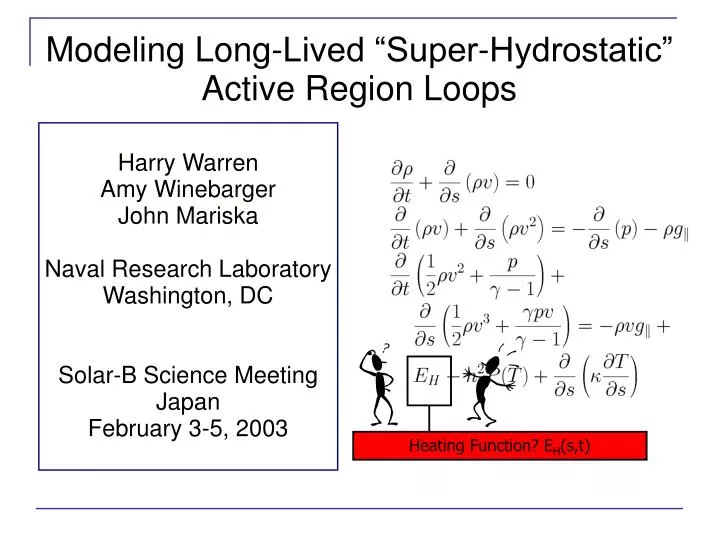
Heating Function? EH(s,t) Modeling Long-Lived “Super-Hydrostatic” Active Region Loops Harry Warren Amy Winebarger John Mariska Naval Research Laboratory Washington, DC Solar-B Science Meeting Japan February 3-5, 2003
Motivation: Understanding the properties of active region loops observed with TRACE Aschwanden et al., 2001, ApJ, v550, p1036
Static Models Don’t Work! • RTVS (uniform heating) scaling law predicts very low densities for long loops. • TRACE observations show nobs/nuni ~ 100! • RTVS (foot point heating) scaling law gives densities that are higher, but only by a factor of about ~3. • Highly localized footpoint heating → instability. Winebarger et al., ApJ, in press
Cargill et al., 1995, ApJ, 439, 1034 Rosner et al., 1978, ApJ, 220, 643 Dynamic solutions can be much denser than static solutions Warren et al., 2002, ApJL, v570, p41
Delay between the appearance of the loop in 195 and 171 Simulated TRACE light curves
4-Jul-1998 (Aschwanden Loop #23) Winebarger et al., ApJ, submitted
Simulated loop cools too fast! EF = 2 ergs cm-3 s-1, δ = 680 s
Not one loop, many filaments? – Consistent with the light curve 10 filaments, EF ≈ 0.2-2 ergs cm-3 s-1, δ = 680 s
SXT/TRACE intensity ratios are consistent with filamentation
Conclusions/Implications for Solar-B • Dynamics and filamentation are important in determining what is observed • EIS+XRT+SOT will provide an unprecedented opportunity to study the dynamical evolution of active region loops • More modeling is needed to identify signatures of coronal heating