Download
1 / 24
240 likes | 327 Vues
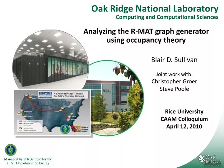
Oak Ridge National Laboratory Computing and Computational Sciences. Analyzing the R-MAT graph generator using occupancy theory. Blair D. Sullivan Joint work with: Christopher Groer Steve Poole. Rice University CAAM Colloquium April 12, 2010. R-MAT: a Recursive MATrix generator.

E N D
Oak Ridge National LaboratoryComputing and Computational Sciences Analyzing the R-MAT graph generator using occupancy theory Blair D. Sullivan Joint work with:Christopher Groer Steve Poole Rice University CAAM Colloquium April 12, 2010
R-MAT: a Recursive MATrix generator • Introduced by Chakrabarti, Faloutsos, Zhan (2004) as a “scale-free” digraph generator (power law degree distribution). • Recursively partitions the adjacency matrix of a graph G according to four probabilities to select position of an edge. The number of vertices must be a power of two, say n = 2k. • Repeats process M times, and may choose an edge multiple times. Duplicates are discarded at the end to form G’ with M’ distinct edges. • Used in many applications, including the SSCA#2 HPC benchmark.
Generating an edge in R-MAT • Let α + β + γ + δ = 1. • Edges are generated by recursively using parameters to choose a location in the adjacency matrix. • Alternatively, you can think of each choice as specifying a pair of digits in the binary representations of the edge endpoints.
Edge probabilities • For the remainder of this talk, we will think of the vertices of G as length-k binary strings. • Let the eα, eβ, eγ, and eδ be the number of positions in the paired binary representations of an edge’s endpoints corresponding to (0,0), (0,1), (1,0), and (1,1), respectively. • Example: e = (u,v) in a graph with 26 vertices. eα= 1 eβ = 2 eγ = 1 eδ= 2 u = 0 0 0 1 1 1 v = 0 1 1 0 1 1 • The probability of generating e is then:
More on edge probabilities • We proved the probability of generating any edge that starts at a vertex u depends solely on the number of zeros in u’s binary string, say uz. • Let λ = α + β and μ = α + γ be the probabilities of choosing “up” and “left” in the matrix, respectively. • Given a vertex u, one can show the probability of an edge of the form (u,v) for some v is: • Similarly, the probability of an edge (v,u) is:
Results for the R-MAT multi-graph • R-MAT naturally generates a multi-graph before duplicate edges are removed. • The probability of out-degree d is binomial: • The expected number of vertices with out-degree d is: • The probability distribution for the total degree is given by:
Total Degree Distribution w/ Duplicates α = β = γ = δ = .25 α = .55, β = γ = .1, δ = .25 Note that the total degree distribution varies with the choice of your quadrant probabilities. α = δ = .15, β = .5, γ = .2 n = 26 vertices, M = 29 edges
Duplicate Removal (an illustration) n = 26 vertices, M = 29 edges, M’ ~ 28.4 edges α = .55, β = γ = .1, δ = .25
Balls and Urns • A classical occupancy problem is often described in terms of tossing r indistinguishable balls into m distinguishable urns and finding the probability that exactly n of these urns are non-empty. • The R-MAT generator can be modeled as such a problem by envisioning the 4k positions in the adjacency matrix as the set of urns, and the M randomly generated edges as the set of balls tossed into these urns. The number of edges M’ in the graph G’ then corresponds to the number of non-empty urns.
Balls and Annoyingly-Unequal Urns • Traditionally, when throwing balls into urns, the probability of “hitting” every urn is the same. R-MAT matrix positions have unequal probabilities, so let q = {q1, q2, …, qm} be the urn probabilities. • Let U(r, l, m, q, t) be the probability that exactly t of the first l urns are empty after tossing r balls into the set of m urns with probability vector q. • Johnson & Kotz proved: • Note this quantity is independent of the ordering of elements in q.
The Easy Answer • One can now derive an expression for the probability of outdegree d by letting = {p(uv)} v=0,1,…n-1: • Note that since the function U is independent of the ordering of , this quantity is the same for all vertices u with a given value of uz. • Unfortunately, this is not a computationally convenient formula.
Using the “Big Urn” • A straightforward corollary to Johnson & Kotz allows us to calculate U when l is not equal to m: • We can now think of throwing balls into the 2k urns in a row plus a “big urn” encompassing all other possible edges, with probability 1 - . Let be the vector obtained by appending 1- to . Then,
Out-degree and binary representation KEY FACT: The out-degree distribution of a vertex is completely determined by the parameters k, M, α, β, γ, δ, and the number of zeros in its binary representation (uz). The exact out-degree distribution for the 7 values of uz & the overall out-degree distribution for a 64-node graph with M = 8*64 and α = .55, β = γ = .1, δ = .25.
Computational Complexity • Problem: calculating the out-degree distribution using these formulas requires massive amounts of computation, e.g. a naïve approach requires O(267) operations for a 64-node graph! • Solution: we analyzed the limiting distributions. • There has been a lot of work on the necessary conditions on a set of probability vectors to get certain distributions. For example, when the probabilities are all equal, the limiting distribution is Poisson.
Applying Chistyakov’s Theorem Theorem (Chistyakov, 1964) Given a set of m urns with probabilities q = {q1, q2, …, qm} which sum to 1, let X be the r.v. corresponding to the number of empty urns after tossing r balls. Then if r, m tend to ∞ with r/m → C1(non-negative and finite), and m ∙ qi≤ C2 < ∞ for each i, then X ~ N(E[X], Var[X])
Applying Chistyakov’s Theorem Theorem (Chistyakov, 1964) Given a set of m urns with probabilities q = {q1, q2, …, qm} which sum to 1, let X be the r.v. corresponding to the number of empty urns after tossing r balls. Then if r, m tend to ∞ with r/m → C1(non-negative and finite), and m ∙ qi≤ C2 < ∞ for each i, then X ~ N(E[X], Var[X]) • We first proved a corollary showing that the number of empty urns among the first m-1 of the m urns is also asymptotically normally distributed with the expected mean and variance.
Applying Chistyakov’s Theorem Theorem (Chistyakov, 1964) Given a set of m urns with probabilities q = {q1, q2, …, qm} which sum to 1, let X be the r.v. corresponding to the number of empty urns after tossing r balls. Then if r, m tend to ∞ with r/m → C1(non-negative and finite), and m ∙ qi≤ C2 < ∞ for each i, then X ~ N(E[X], Var[X]) • We first proved a corollary showing that the number of empty urns among the first m-1 of the m urns is also asymptotically normally distributed with the expected mean and variance. • Assuming that the ratio of r to m is bounded (m= O(n)), it remains to prove that m∙qi≤ C2 <∞ for each i. In the case of R-MAT, for every vertex u, we need to show n ∙ p(uv) → cv for all vertices v.
Proving n∙p(uv) → cv • Case 1: 0 < α, β, γ, δ ≤ 0.5 • This is straightforward, as the quantityn∙p(uv) is uniformly bounded above by the constant 1. • Case 2: 0 < min(α, β, γ, δ) & max(α, β, γ, δ) > 0.5 • We were able to prove that all but a vanishing proportion of the vertices satisfy the necessary criterion: • This requires the use of Chebyshev’s inequality to prove the limit of a weighted sum of binomial coefficients.
Limiting Distributions • These results allow us to prove that the limiting distributions for in-, out-, and total-degree are asymptotically normal when all parameters are strictly positive and M = O(n) : • The overall degree distribution for G’ is thus a mixture of normal distributions (one for each value of uz).
Experimental Evidence (for approximations) Comparison of observed versus limiting distribution, averaged over 2048 graphs with n = 212 and M = 217.
How many duplicate edges were there? • We can also approximate the variance of M’. We believe M’ is normally distributed, but this is still an open problem. This is a histogram of the observed values of M’ for 216 graphs generated with n = 220, M = 223 and R-MAT parameters α = .55, β = γ = .1, δ = .25. The red line shows a normal distribution with mean and variance calculated according to our formulas.
Graph Compression Algorithms Joint work with Chris Groer, Steve Poole Funded by Department of Defense • Development of consistent representations and metrics for compression. • Computational study comparing variants of MDL (minimum description length) and binary matrix reordering (TSP)-based algorithms. • Proved finding optimal MDL representation is NP-hard & formulated as a mixed integer program.
Graph Decompositions and Petascale Data Joint work with Chris Groer Funded by DOE Office of Advanced Scientific Computing Research • Objective: Leverage theoretical work on graph decompositions to create efficient computational framework for graph-based data. • Approach: • Low width decompositions of sparse application graphs • Algorithm complexity becomes exponential in width, but polynomial in number of nodes • Integrate parallel computing with decompositions for massive graph analysis • Challenges: • Low width decompositions are insufficient • Need to control structure of the decomposition (balanced bag sizes & tree far from being a path) • Modify dynamic programming to run in parallel
Acknowledgements This work was supported by the United States Department of Defense and the United States Department of Energy’s Office of Advanced Scientific Computing Research (OASCR). Resources of the Extreme Scale Systems Center at Oak Ridge National Laboratory were used for computational results.