Download
1 / 49
490 likes | 583 Vues
Transition of Component States. Normal state continues. Component fails. Failed state continues. N. F. Component is repaired. The Repair-to-Failure Process. Definition of Reliability.

E N D
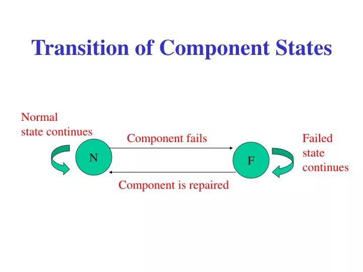
Transition of Component States Normal state continues Component fails Failed state continues N F Component is repaired
Definition of Reliability • The reliability of an item is the probability that it will adequately perform its specified purpose for a specified period of time under specified environmental conditions.
REPAIR -TO-FAILURE PROCESS MORTALITY DATA t=age in years ; L(t) =number of living at age t t L(t) t L(t) t L(t) t L(t) 0 1,023,102 15 962,270 50 810,900 85 78,221 1 1,000,000 20 951,483 55 754,191 90 21,577 2 994,230 25 939,197 60 677,771 95 3,011 3 990,114 30 924,609 65 577,822 95 125 4 986,767 35 906,554 70 454,548 5 983,817 40 883,342 75 315,982 10 971,804 45 852,554 80 181,765 After Bompas-Smith. J.H. Mechanical Survival : The Use of Reliability Data, McGraw-Hill Book Company, New York , 1971.
HUMAN RELIABILITY t L(t), Number Living at Age in Years Age t R(t)=L(t)/N F(t)=1-R(t) repair= birth failure = death Meaning of R(t): (1) Prob. Of Survival (0.87) of an individual of an individual to age t (40) (2) Proportion of a population that is expected to Survive to a given age t. 0 1,023,102 1. 0. 1 1,000,000 0.9774 0.0226 2 994,230 0.9718 0.0282 3 986,767 0.9645 0.0322 4 983,817 0.9616 0.0355 5 983,817 0.9616 0.0384 10 971,804 0.9499 0.0501 15 962,270 0.9405 0.0595 20 951,483 0.9300 0.0700 25 939,197 0.9180 0.0820 30 924,609 0.9037 0.0963 40 883,342 0.8634 0.1139 45 852,554 0.8333 0.1667 50 810,900 0.7926 0.2074 55 754,191 0.7372 0.2628 60 677,771 0.6625 0.3375 65 577,882 0.5648 0.4352 70 454,548 0.4443 0.5557 75 315,982 0.3088 0.6912 80 181,765 0.1777 0.8223 85 78,221 0.0765 0.9235 90 21,577 0.0211 0.9789 95 3,011 0.0029 0.9971 99 125 0.0001 0.9999 100 0 0. 1.
1.0 0.9 0.8 0.7 0.6 0.5 0.4 0.3 0.2 0.1 Probability of Survival R(t) and Death F(t) Reliability, R(t) = probability of survival to (inclusive) age t = the number of surviving at t divided by the total sample Unreliability, F(t) = probability of death to age t (t is not included) =the total number of death before age t divided by the total population 0 10 20 30 40 50 60 70 80 90 100 Figure 4.3 Survival and failure distributions.
1.0 P 0.9 Survival distribution 0.8 0.7 0.6 0.5 Probability of Survival R(t) and Death F(t) 0.4 0.3 Failure distribution 0.2 0.1 0 10 20 30 40 50 60 70 80 90 100
FALURE DENSITY FUNCTION f(t) No. of Failures (death) Age in Years 0.02260 0.00564 0.00402 0.00327 0.00288 0.00235 0.00186 0.00211 0.00240 0.00285 0.00353 0.00454 0.00602 0.00814 0.01110 0.01500 0.01950 0.02410 0.02710 0.02620 0.02020 0.01110 0.00363 0.00071 000012 0 1 2 3 4 5 10 15 20 25 30 35 40 45 50 60 65 70 75 80 85 90 95 99 100 23,102 5,770 4,116 3,347 2,950 12,013 9,543 10,787 12,286 14,588 18,055 23,212 30,788 41,654 56,709 99,889 123,334 138,566 134,217 103,554 56,634 18,566 2,886 125 0 0.00540 0.00454 0.00284 0.00330 0.00287 0.00192 0.00198 0.00224 0.00259 0.00364 0.00393 0.00436 0.00637 0.00962 0.01367 0.01800 0.02200 0.02490 0.02610 0.02460 0.01950 0.00970 0.00210 - - -
140 120 100 80 60 40 20 0.14 0.12 0.10 0.8 0.6 0.4 0.2 0.0 Numbre of Deaths (thousands) Failure Density f(t) 0 20 40 60 80 100 0 20 40 60 80 100 Age in Years (t) Figure 4.4 Histogram and smooth curve
140 120 100 80 Number of Deaths (thousands) 60 40 20 Age in Years (t) 20 40 60 80 100
0.14 0.12 0.10 Failure Density f (t) 0.8 0.6 0.4 0.2 Age in Years (t) 20 40 60 80 100
CALCULATION OF FAILURE RATE r(t) Age in Years No. of Failures (death) Age in Years No. of Failures (death) r(t)= r(t)= 0 1 2 3 4 5 10 15 20 25 30 35 23,102 5,770 4,116 3,347 2,950 12,013 9,534 10,787 12,286 14,588 18,055 23,212 0.02260 0.00570 0.00414 0.00338 0.00299 0.00244 0.00196 0.00224 0.00258 0.00311 0.00391 0.0512 40 45 50 55 60 65 70 75 80 85 90 95 99 30,788 41,654 56,709 76,420 99,889 123,334 138,566 134,217 103,554 56,634 18,566 2,886 125 0.00697 0.00977 0.01400 0.02030 0.02950 0.04270 0.06100 0.08500 0.11400 0.14480 0.17200 0.24000 1.20000
Random failures 0.2 0.15 0.1 0.05 Wearout failures Failure rate f (t) 0 20 40 60 80 100 t,years Bathtub Curve Figure 4.6 Failure rate r (t) versus t.
Random failures Early failures Wearout failures 0.2 0.15 Failure Rate r(t) 0.1 0.05 20 40 60 80 100 Failure rate r(t) versus t.
Reliability - R(t) • The probability that the component experiences no failure during the the time interval (0,t). • Example: exponential distribution
Unreliability - F(t) • The probability that the component experiences the first failure during (0,t). • Example: exponential distribution
Failure Density - f(t) (exponential distribution)
Failure Rate - r(t) • The probability that the component fails per unit time at time t, given that the component has survived to time t. • Example: The component with a constant failure rate is considered as good as new, if it is functioning.
Failure Rate Failure Density Unreliability Reliability 1 1 Area = 1 1 - F (t) f (t) F (t) R (t) 0 0 t (a) t (b) t (c) t (d) Figure 11-1 Typical plots of (a) the failure rate (b) the failure density f (t), (c) the unreliability F(t), and (d) the reliability R (t).
Failure Rate, (faults/time) Period of Approximately Constant failure rate Infant Mortality Old Age Time Figure 11-2 A typical “bathtub” failure rate curve for process hardware. The failure rate is approximately constant over the mid-life of the component.
TABLE 11-1: FAILURE RATE DATA FOR VARIOUS SELECTED PROCESS COMPONENTS1 Instrument Fault/year Controller 0.29 Control valve 0.60 Flow measurement (fluids) 1.14 Flow measurement (solids) 3.75 Flow switch 1.12 Gas - liquid chromatograph 30.6 Hand valve 0.13 Indicator lamp 0.044 Level measurement (liquids) 1.70 Level measurement (solids) 6.86 Oxygen analyzer 5.65 pH meter 5.88 Pressure measurement 1.41 Pressure relief valve 0.022 Pressure switch 0.14 Solenoid valve 0.42 Stepper motor 0.044 Strip chart recorder 0.22 Thermocouple temperature measurement 0.52 Thermometer temperature measurement 0.027 Valve positioner 0.44 1Selected from Frank P. Lees, Loss Prevention in the Process Industries (London: Butterworths, 1986), p. 343.
A System with n Components in Parallel • Unreliability • Reliability
A System with n Components in Series • Reliability • Unreliability
Upper Bound of Unreliability for Systems with n Components in Series
Pressure Switch Alarm at P > PA PIA PIC Pressure Feed Solenoid Valve Reactor Figure 11-5 A chemical reactor with an alarm and inlet feed solenoid. The alarm and feed shutdown systems are linked in parallel.
Alarm System • The components are in series Faults/year years
Shutdown System • The components are also in series:
The Overall Reactor System • The alarm and shutdown systems are in parallel:
Repair Probability - G(t) • The probability that repair is completed before time t, given that the component failed at time zero. • If the component is non-repairable
Repair Rate - m(t) • The probability that the component is repaired per unit time at time t, given that the component failed at time zero and has been failed to time t. • If the component is non-repairable
Availability - A(t) • The probability that the component is normal at time t. • For non-repairable components • For repairable components
Unavailability - Q(t) • The probability that the component fails at time t. • For non-repairable components • For repairable components
Unconditional Repair Density, w(t) The probability that a component fails per unit time at time t, given that it jumped into the normal state at time zero. Note, for non-repairable components.
Unconditional Repair Density, v(t) The probability that the component is repaired per unit time at time t, give that it jumped into the normal state at time zero.
Conditional Failure Intensity, λ(t) The probability that the component fails per unit time, given that it is in the normal state at time zero and normal at time t. In general , λ(t)≠r(t). For non-repairable components, λ(t) = r(t). However, if the failure rate is constant (λ) , then λ(t) = r(t) = λ for both repairable and non-repairable components.
Conditional Repair Intensity, µ(t) The probability that a component is repaired per unit time at time t, given that it is jumped into the normal state at time zero and is failed at time t, For non-repairable component, µ(t)=m(t)=0. For constant repair rate m, µ(t)=m.
ENF over an interval, W(t1,t2 ) Expected number of failures during (t1,t2) given that the component jumped into the normal state at time zero. For non-repairable components
SHORT-CUT CALCULATION METHODS Information Required Approximation of Event Unavailability When time is long compared with MTTR and , the following approximation can be made, Where, is the MTTR of component j.
Z AND X Y IF X and Y are Independent
Z OR X Y
COMPUTATION OF ACROSS LOGIC GATES AND GATES OR GATES
CUT SET IMPORTANCE The importance of a cut set K is defined as Where, is the probability of the top event. may be interpreted as the conditional probability that the cut set occurs given that the top event has occurred. PRIMAL EVENT IMPORTANCE The importance of a primal event is defined as or Where, the sum is taken over all cut sets which contain primal event .
[ EXAMPLE ] As an example , consider the tree used in the section on cut sets. The cut sets for this tree are (1) , (2) , (6) , (3,4) ,(3,5). The following data are given from which we compute the unavailabilities for each event. 1 .16 1.5E-5 (.125) 2.4E-6 2 .2 1.5E-5 (.125) 3.0E-6 3 1.4 7E-4 (6) 9.8E-4 4 30 1.1E-4 (1) 3.3E-3 5 5 1.1E-4 (1) 5.5E-4 6 .5 5.5E-5 (.5) 2.75E-5 Now, compute the probability of occurrence for each cut set and top event probability. (1) 2.4E-6 (2) 3.0E-6 (6) 2.75E-5 (3,4) 3.23E-6 (3,5) 5.39E-7 3.67E-5