Download
1 / 22
220 likes | 453 Vues
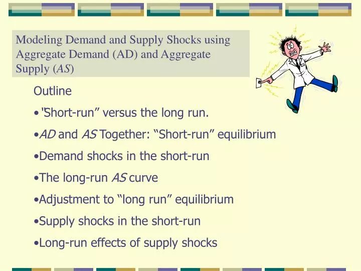
Modeling Demand and Supply Shocks using Aggregate Demand (AD) and Aggregate Supply ( AS ). Outline “ Short-run” versus the long run. AD and AS Together: “Short-run” equilibrium Demand shocks in the short-run The long-run AS curve Adjustment to “long run” equilibrium

E N D
Modeling Demand and Supply Shocks using Aggregate Demand (AD) and Aggregate Supply (AS) • Outline • “Short-run” versus the long run. • AD and AS Together: “Short-run” equilibrium • Demand shocks in the short-run • The long-run AS curve • Adjustment to “long run” equilibrium • Supply shocks in the short-run • Long-run effects of supply shocks
Professors Hall and Lieberman call the Keynesian model a “short-run” model. Why? Because it is possible for the economy to be in equilibrium, but at the same time real GDP can be above or below potential or full employment GDP
Long-run equilibrium occurs when the economy is in equilibrium at full employment • Point K is a short-run equilibrium since Y1 < YFE • Point H is a short-run equilibrium since Y2 > YFE • Point E is a long-run equilibrium since equilibrium GDP corresponds to YFE AE AE3 H AE2 AE1 E Full employment GDP K 450 Real GDP($Trillions) Y1 YFE Y2 0
Short run equilibrium is a combination of price level and GDP consistent with both AS and AD curves
At point B, the price level is 140 and AS = $14 trillion. But equilibrium GDP is equal to $6 trillion when the price level is 140—we know this from the AD curve. • At point E, the price level is consistent with an output level of $10 along bothAS and AD curves Why is point E a short-run equilibrium? PriceLevel AS B 140 E 100 F AD 0 6 10 14 Real GDP($Trillions)
Effect of a Demand Shock Issue: Why did the economy move from point E to point H—instead of E to J? Increase in government spending PriceLevel AS 130 J H 100 E AD2 AD1 0 10 12 13.5 Real GDP($Trillions)
AD curve shifts rightward Multiplier Effect G GDP Movement along new AD curve Unit cost Money Demand Interest rate a and IP P GDP Movement along AS curve Net result: GDP increases, but by less due to the effect of an increase in the price level
Effect of a decrease in the money supply PriceLevel AS K 100 E S AD2 AD1 0 6.5 8 10 Real GDP($Trillions)
AD curve shifts Leftward Interest rate a and IP M GDP Movement along new AD curve Unit cost Money Demand Interest rate a and IP P GDP Movement along AS curve Net result: GDP decreases, but by less due to the effect of an decrease in the price level
Long run aggregate supply PriceLevel Long run AS curve Long run AS curve: A vertical line indicating all possible output and price level combinations the economy could end up in the long run 0 YFE Real GDP($Trillions)
Self correcting mechanism (How does it work?) Some economists (including Hall & Lieberman) believe the economy is “self-correcting”—that is, forces are present that push the economy to long-run (or full-employment) equilibrium.
Long Run AS Curve AS2 PriceLevel AS1 Let AD shift from AD1 to AD2 P4 K P3 J P2 H P1 E AD2 AD1 0 YFE Y3 Y2 Real GDP($Trillions)
Change in short-run equilibrium Positive demand shock P and Y Y until Y =YFE Wage Rate Y > YFE Unit Cost P Long-run adjustment process
Supply shocks • The following factors could shift the (short-run) aggregate supply schedule up to the left: • An increase in the price of a basic commodity—e.g., petroleum, natural gas, wheat, soybeans. • An increase in average money wages and benefits not restricted to just one industry or sector of the economy. • An increase in the average markup over unit cost not restricted to just one industry or sector of the economy.
Effect of an increase in petroleum prices PriceLevel AS2 AS1 S 130 100 E AD2 AD1 0 6.5 8 10 Real GDP($Trillions)
I’d call that a shock, wouldn’t you? The storyof Joseph (see Old Testament)suggests buffer stocksas the remedy forsupply-shockinflation 1970s Oil Shock Price of One Barrel of 340 crude oil Source: The Petroleum Economist
Defining Productivity Productivity() means the average output of a workerper year, or alternatively: = GDP/Nwhere N is total employment and Y is real GDP. depends onthe efficiency withwhich labor is employedin the production ofgoods & services
Productivity and cost Let denote average annual compensation of employees (including benefits). Thus unit labor cost (UCL) is defined as: ULC = / Notice that compensationcan rise with no effect on ULC, so long as productivitykeeps pace
Source: www.dismal.com % change, annual rate