Download

1 / 19
190 likes | 201 Vues
Query Processing and Optimization. Objectives. Introduction + Major Phases in Query Processing + Optimizing Queries + Steps in Query Optimization + Query Trees and Graphs + Relational Algebra Transformation + Query Processing and Optimization +. - Introduction.

E N D
Query Processing and Optimization Databases: Query Proc. & Opt.
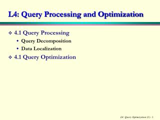
Objectives • Introduction + • Major Phases in Query Processing + • Optimizing Queries + • Steps in Query Optimization + • Query Trees and Graphs + • Relational Algebra Transformation + • Query Processing and Optimization + Databases: Query Proc. & Opt.
- Introduction • With declarative languages such as SQL, the user specifies what data is required rather than how it is retrieved • Relieves user of knowing what constitutes a good execution strategy • Also gives the DBMS more control over system performance. Databases: Query Proc. & Opt.
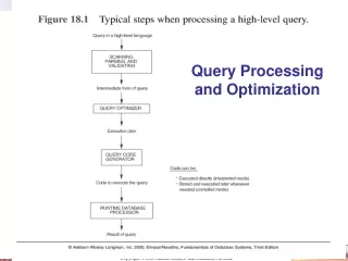
-- Processing a High-Level Query Query in high level language Scanning, parsing And Validating Intermediate form of query Query Optimizer Execution plan Query code Generator Code to execute the query Run time DB Processor Query result Databases: Query Proc. & Opt.
- Major Phases in Query Processing • Scan, Parse, and Validate Query: Transform query written in high level language (e g. SQL), into correct efficient execution strategy expressed in low-level language (e. g. Relational Algebra) • Optimize query and generate code: produce an execution strategy or plan and run-time code. • Execute query: Implement the plan to retrieve required data. Databases: Query Proc. & Opt.
- Optimizing Queries • The objective in query optimization is to select an efficient execution strategy. • As there are many equivalent transformations from same high-level query, aim is to choose the one that minimizes resource usage. • Generally, an efficient execution plan reduces the total execution time of a query; thereby reducing the response time of a query. • The problem is computationally intractable with large number of relations, so the strategy adopted is reduced to finding a near optimum solution. • Two main techniques for query optimization are: • Heuristic rules that order operations in a query • Comparing different strategies based on relative cost, and selecting one that minimizes resource usage. Databases: Query Proc. & Opt.
- Steps in Query Optimization • In using heuristics during query optimization, the following steps must be followed: • Translate queries into query trees or query graphs • Apply transformation rules for relational algebra expression. • Perform heuristic optimization Databases: Query Proc. & Opt.
-- Query Trees and Graphs • A query tree is a tree data structure that corresponds to a relational algebra expression. It represents the input relations of the query as leaf nodes of the tree, and represents the relational algebra operations as internal nodes • An execution of the query tree consists of executing an internal node operation whenever its operands are available and then replacing that internal node by the relation that results from executing the operation. • The execution terminates when the root node is executed and produces the result relation for the query. Databases: Query Proc. & Opt.
--- Query Tree Example … • For every project located in ‘Stafford’, list the project number, the controlling department number and the department manager’s last name, address, and birth date. SELECT Pnumber, Dnum, Lname, Address, Bdate FROM Project, Department, Employee WHERE Dnum=Dnumber AND MgrSSN = SSN AND Plocation = ‘Stafford’ • Equivalent relational algebra expression is: ∏Pnumber, Dnum, Lname, Address, Bdate (((σPlocation = ‘Stafford’(Project)) θDnum=Dnumber(Department)) θMgrSSN=SSN(Employee)) Note: θ stands for JOIN Databases: Query Proc. & Opt.
… --- Query Tree: Example ∏P.Pnumber, P.Dnum, E.Lname, E.Address, E.Bdate θD.MGRSSN=E.SSN θP.Dnum=D.Dnumber Employee E σP.Location=‘Stafford’ Department D Project P Note: The symbol θrepresents JOIN Databases: Query Proc. & Opt.
… --- Query Tree: Example ∏P.Pnumber, P.Dnum, E.Lname, E.Address, E.Bdate σP.Dnum=D.Dnumber AND D.MGRSSN=E.SSN AND P.Location=‘Stafford’ Χ X E D P Databases: Query Proc. & Opt.
- Relational Algebra Transformation … • The following list gives a basic selection of relational algebra transformation: • Cascade of selection: Conjunctive selection operations can cascade into individual selection operations p AND q AND r (R) = p (q (r (R))) • Cascade of projection: In a sequence of projection operations, only the last in sequence is required. L(M(…(N(R) = L(R) • Commutatively of selection: A sequence of selection operations are commutative q(p(R)) = p(q(R)) • Associativity of Natural Join and Cross Product: Natural join (*) and Cross Product (X) are associative: (R * S) * T = R * (S * T) (R X S) X T = R X (S X T) Databases: Query Proc. & Opt.
-- Heuristic Optimization • Perform selection operations as early as possible • Keep predicates on same relation together • Combine Cartesian product with subsequent selection whose predicate represents join condition into a join operation. • Use associative of binary operations to rearrange leaf nodes with most restrictive selection operations first. • Perform projection as early as possible • Keep projection attributes on same relations together. • Compute common expressions once. • If common expression appears more than once, and result not too large, store result and reuse it when required. • Useful when querying views, as same expression is used to construct view each time. Databases: Query Proc. & Opt.
-- Query Optimization: Example … • Query: Find the last name of employees born after 1975 who work on a project named ‘Aquarius’ SELECT Lname FROM Employee, Works_on, Project WHERE Pname = ‘Aquarius’ AND ESSN = SSN AND Pnumber = PNO AND Bdate > ‘1975-12-31’ Databases: Query Proc. & Opt.
… -- Query Optimization: Example … ∏Lname σPname=‘Aquirius’ AND P.Number=PNO AND ESSN=SSN AND Bdate=‘Dec-31-1957’ Χ Initial Canonical Query Tree X Project Works_On Employee Databases: Query Proc. & Opt.
… -- Query Optimization: Example … ∏Lname σPnumber=PNO Moving SELECT down Χ σPname=‘Aquarius’ σESSN=SSN X Project σBDate=‘1957-12-13’ Works_On Employee Databases: Query Proc. & Opt.
… -- Query Optimization: Example … ∏Lname σESSN=SSN Apply more restrictive SELECT Χ σBDate=‘1957-12-13’ σPnumber=PNO X Employee σPname=‘Aquirius’ Works_On Project Databases: Query Proc. & Opt.
… -- Query Optimization: Example … ∏Lname Replace CARTESIAN PRDUCT And SELECT with JOIN σESSN=SSN σBDate=‘1957-12-13’ θPnumber=Pno σPname=‘Aquirius’ Employee Works_On Project Databases: Query Proc. & Opt.
… -- Query Optimization: Example ∏Lname Move PROJECTION down θESSN=SSN ∏SSN,Lname ∏ESSN θPnumber=Pno σBDate=‘1957-12-13’ ∏ESSN,PNO ∏Pnumber Employee σPname=‘Aquirius’ Works_On Project Databases: Query Proc. & Opt.