Download
1 / 17
180 likes | 279 Vues
Using “vlookup” function in Excel to complete “Days Enrolled”. Howard De Leeuw , OSPI howard.deleeuw@k12.wa.us 360-725-6147. Open both your downloaded file and your newly-created “Days Enrolled” file in Excel. In your downloaded file, click in the first cell under the “DAYS_ENR” column.

E N D
Using “vlookup” function in Excel to complete “Days Enrolled” Howard De Leeuw, OSPI howard.deleeuw@k12.wa.us 360-725-6147
Open both your downloaded file and your newly-created “Days Enrolled” file in Excel
In your downloaded file, click in the first cell under the “DAYS_ENR” column
Go to “Insert Function” search for “vlookup”, highlight it and click “OK”
A “function arguments” window will open – click on the icon next to the “Lookup_value” field
Select the entire “EDATE” column, then click on the icon at the far right of the “Function Arguments” window
Now back at the main window, click on the icon at the end of the “Table_array” field.
Now go to your “Days Enrolled” file that you created and select both the “Date” and “Day” columns, then click the icon on the far right.
You are now back to your main file and main “Function Arguments” window. Enter “2” in the Col_index_num” field
In the “Range_lookup” field enter “false” and then click “OK” at the bottom of the window.
If everything went as planned, you should see a number of days in the cell.
Now you need to drag the formula from the first cell to the bottom of your spreadsheet – this will then apply the calculation to every cell.
When the “Paste Special” window opens, select “Values” and click OK – this will preserve your data and remove the formula.