Download
1 / 55
550 likes | 556 Vues
CSC401 – Analysis of Algorithms Chapter 6 Graphs. Objectives: Introduce graphs and data structures Discuss the graph connectivity and biconnectivity Present the depth-first and breath-first search algorithms as well as algorithms for finding biconnected components

E N D
CSC401 – Analysis of Algorithms Chapter 6Graphs Objectives: Introduce graphs and data structures Discuss the graph connectivity and biconnectivity Present the depth-first and breath-first search algorithms as well as algorithms for finding biconnected components Introduce directed graphs and algorithms performed on directed graphs: Reachability, transitive closure, DAG CSC401: Analysis of Algorithms
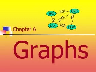
A graph is a pair (V, E), where V is a set of nodes, called vertices E is a collection of pairs of vertices, called edges Vertices and edges are positions and store elements Example: A vertex represents an airport and stores the three-letter airport code An edge represents a flight route between two airports and stores the mileage of the route 849 PVD 1843 ORD 142 SFO 802 LGA 1743 337 1387 HNL 2555 1099 1233 LAX 1120 DFW MIA Graph CSC401: Analysis of Algorithms
flight AA 1206 ORD PVD 849 miles ORD PVD Edge Types • Directed edge • ordered pair of vertices (u,v) • first vertex u is the origin • second vertex v is the destination • e.g., a flight • Undirected edge • unordered pair of vertices (u,v) • e.g., a flight route • Directed graph • all the edges are directed • e.g., route network • Undirected graph • all the edges are undirected • e.g., flight network CSC401: Analysis of Algorithms
V a b h j U d X Z c e i W g f Y Terminology • End vertices (or endpoints) of an edge • U and V are the endpoints of a • Edges incident on a vertex • a, d, and b are incident on V • Adjacent vertices • U and V are adjacent • Degree of a vertex • X has degree 5 • Parallel edges • h and i are parallel edges • Self-loop • j is a self-loop CSC401: Analysis of Algorithms
Terminology (cont.) • Path • sequence of alternating vertices and edges • begins with a vertex • ends with a vertex • each edge is preceded and followed by its endpoints • Simple path • path such that all its vertices and edges are distinct • Examples • P1=(V,b,X,h,Z) is a simple path • P2=(U,c,W,e,X,g,Y,f,W,d,V) is a path that is not simple V b a P1 d U X Z P2 h c e W g f Y CSC401: Analysis of Algorithms
V a b d U X Z C2 h e C1 c W g f Y Terminology (cont.) • Cycle • circular sequence of alternating vertices and edges • each edge is preceded and followed by its endpoints • Simple cycle • cycle such that all its vertices and edges are distinct • Examples • C1=(V,b,X,g,Y,f,W,c,U,a,) is a simple cycle • C2=(U,c,W,e,X,g,Y,f,W,d,V,a,) is a cycle that is not simple CSC401: Analysis of Algorithms
Notation n number of vertices m number of edges deg(v)degree of vertex v Property 1 Sv deg(v)= 2m Proof: each edge is counted twice Property 2 In an undirected graph with no self-loops and no multiple edges m n (n -1)/2 Proof: each vertex has degree at most (n -1) What is the bound for a directed graph? Properties Example • n = 4 • m = 6 • deg(v)= 3 CSC401: Analysis of Algorithms
Vertices and edges are positions store elements Accessor methods aVertex() incidentEdges(v) endVertices(e) isDirected(e) origin(e) destination(e) opposite(v, e) areAdjacent(v, w) Update methods insertVertex(o) insertEdge(v, w, o) insertDirectedEdge(v, w, o) removeVertex(v) removeEdge(e) Generic methods numVertices() numEdges() vertices() edges() Main Methods of the Graph ADT CSC401: Analysis of Algorithms
Edge List Structure • Vertex object • element • reference to position in vertex sequence • Edge object • element • origin vertex object • destination vertex object • reference to position in edge sequence • Vertex sequence • sequence of vertex objects • Edge sequence • sequence of edge objects u a c b d v w z z w u v a b c d CSC401: Analysis of Algorithms
Adjacency List Structure • Edge list structure • Incidence sequence for each vertex • sequence of references to edge objects of incident edges • Augmented edge objects • references to associated positions in incidence sequences of end vertices a v b u w w u v b a CSC401: Analysis of Algorithms
Adjacency Matrix Structure • Edge list structure • Augmented vertex objects • Integer key (index) associated with vertex • 2D-array adjacency array • Reference to edge object for adjacent vertices • Null for non nonadjacent vertices • The “old fashioned” version just has 0 for no edge and 1 for edge a v b u w 2 w 0 u 1 v b a CSC401: Analysis of Algorithms
Asymptotic Performance CSC401: Analysis of Algorithms
Tree Forest Trees and Forests • A (free) tree is an undirected graph T such that • T is connected • T has no cycles This definition of tree is different from the one of a rooted tree • A forest is an undirected graph without cycles • The connected components of a forest are trees CSC401: Analysis of Algorithms
Spanning Trees and Forests • A spanning tree of a connected graph is a spanning subgraph that is a tree • A spanning tree is not unique unless the graph is a tree • Spanning trees have applications to the design of communication networks • A spanning forest of a graph is a spanning subgraph that is a forest Graph Spanning tree CSC401: Analysis of Algorithms
Depth-first search (DFS) is a general technique for traversing a graph A DFS traversal of a graph G Visits all the vertices and edges of G Determines whether G is connected Computes the connected components of G Computes a spanning forest of G DFS on a graph with n vertices and m edges takes O(n + m ) time DFS can be further extended to solve other graph problems Find and report a path between two given vertices Find a cycle in the graph Depth-first search is to graphs what Euler tour is to binary trees Depth-First Search CSC401: Analysis of Algorithms
DFS Algorithm AlgorithmDFS(G, v) Inputgraph G and a start vertex v of G Outputlabeling of the edges of G in the connected component of v as discovery edges and back edges setLabel(v, VISITED) for all e G.incidentEdges(v) ifgetLabel(e) = UNEXPLORED w opposite(v,e) if getLabel(w) = UNEXPLORED setLabel(e, DISCOVERY) DFS(G, w) else setLabel(e, BACK) • The algorithm uses a mechanism for setting and getting “labels” of vertices and edges AlgorithmDFS(G) Inputgraph G Outputlabeling of the edges of G as discovery edges and back edges for all u G.vertices() setLabel(u, UNEXPLORED) for all e G.edges() setLabel(e, UNEXPLORED) for all v G.vertices() ifgetLabel(v) = UNEXPLORED DFS(G, v) CSC401: Analysis of Algorithms
Property 1 DFS(G, v) visits all the vertices and edges in the connected component of v Property 2 The discovery edges labeled by DFS(G, v) form a spanning tree of the connected component of v A B D E C Properties of DFS CSC401: Analysis of Algorithms
Setting/getting a vertex/edge label takes O(1) time Each vertex is labeled twice once as UNEXPLORED once as VISITED Each edge is labeled twice once as UNEXPLORED once as DISCOVERY or BACK Method incidentEdges is called once for each vertex DFS runs in O(n + m) time provided the graph is represented by the adjacency list structure Recall that Sv deg(v)= 2m Analysis of DFS CSC401: Analysis of Algorithms
Path Finding AlgorithmpathDFS(G, v, z) setLabel(v, VISITED) S.push(v) if v= z return S.elements() for all e G.incidentEdges(v) ifgetLabel(e) = UNEXPLORED w opposite(v,e) if getLabel(w) = UNEXPLORED setLabel(e, DISCOVERY) S.push(e) pathDFS(G, w, z) S.pop(e) else setLabel(e, BACK) S.pop(v) • We can specialize the DFS algorithm to find a path between two given vertices u and z using the template method pattern • We call DFS(G, u) with u as the start vertex • We use a stack S to keep track of the path between the start vertex and the current vertex • As soon as destination vertex z is encountered, we return the path as the contents of the stack CSC401: Analysis of Algorithms
Cycle Finding AlgorithmcycleDFS(G, v, z) setLabel(v, VISITED) S.push(v) for all e G.incidentEdges(v) ifgetLabel(e) = UNEXPLORED w opposite(v,e) S.push(e) if getLabel(w) = UNEXPLORED setLabel(e, DISCOVERY) pathDFS(G, w, z) S.pop(e) else T new empty stack repeat o S.pop() T.push(o) until o= w return T.elements() S.pop(v) • We can specialize the DFS algorithm to find a simple cycle using the template method pattern • We use a stack S to keep track of the path between the start vertex and the current vertex • As soon as a back edge (v, w) is encountered, we return the cycle as the portion of the stack from the top to vertex w CSC401: Analysis of Algorithms
Breadth-first search (BFS) is a general technique for traversing a graph A BFS traversal of a graph G Visits all the vertices and edges of G Determines whether G is connected Computes the connected components of G Computes a spanning forest of G BFS on a graph with n vertices and m edges takes O(n + m ) time BFS can be further extended to solve other graph problems Find and report a path with the minimum number of edges between two given vertices Find a simple cycle, if there is one Breadth-First Search CSC401: Analysis of Algorithms
BFS Algorithm AlgorithmBFS(G, s) L0new empty sequence L0.insertLast(s) setLabel(s, VISITED) i 0 while Li.isEmpty() Li +1new empty sequence for all v Li.elements() for all e G.incidentEdges(v) ifgetLabel(e) = UNEXPLORED w opposite(v,e) if getLabel(w) = UNEXPLORED setLabel(e, DISCOVERY) setLabel(w, VISITED) Li +1.insertLast(w) else setLabel(e, CROSS) i i +1 • The algorithm uses a mechanism for setting and getting “labels” of vertices and edges AlgorithmBFS(G) Inputgraph G Outputlabeling of the edges and partition of the vertices of G for all u G.vertices() setLabel(u, UNEXPLORED) for all e G.edges() setLabel(e, UNEXPLORED) for all v G.vertices() ifgetLabel(v) = UNEXPLORED BFS(G, v) CSC401: Analysis of Algorithms
Notation Gs: connected component of s Property 1 BFS(G, s) visits all the vertices and edges of Gs Property 2 The discovery edges labeled by BFS(G, s) form a spanning tree Ts of Gs Property 3 For each vertex v in Li The path of Ts from s to v has i edges Every path from s to v in Gshas at least i edges Properties A B C D E F L0 A L1 B C D L2 E F CSC401: Analysis of Algorithms
Setting/getting a vertex/edge label takes O(1) time Each vertex is labeled twice once as UNEXPLORED once as VISITED Each edge is labeled twice once as UNEXPLORED once as DISCOVERY or CROSS Each vertex is inserted once into a sequence Li Method incidentEdges is called once for each vertex BFS runs in O(n + m) time provided the graph is represented by the adjacency list structure Recall that Sv deg(v)= 2m Analysis CSC401: Analysis of Algorithms
Applications • Using the template method pattern, we can specialize the BFS traversal of a graph Gto solve the following problems in O(n + m) time • Compute the connected components of G • Compute a spanning forest of G • Find a simple cycle in G, or report that G is a forest • Given two vertices of G, find a path in G between them with the minimum number of edges, or report that no such path exists CSC401: Analysis of Algorithms
DFS: Back edge (v,w) w is an ancestor of v in the tree of discovery edges BFS: Cross edge (v,w) w is in the same level as v or in the next level in the tree of discovery edges L0 A A L1 B C D B C D L2 E F E F DFS DFS vs. BFS BFS CSC401: Analysis of Algorithms
Definitions -- Let G be a connected graph A separation edge of G is an edge whose removal disconnects G A separation vertex of G is a vertex whose removal disconnects G Applications Separation edges and vertices represent single points of failure in a network and are critical to the operation of the network Example DFW, LGA and LAX are separation vertices (DFW,LAX) is a separation edge ORD PVD SFO LGA HNL LAX DFW MIA Separation Edges and Vertices CSC401: Analysis of Algorithms
Biconnected Graph • Equivalent definitions of a biconnected graph G • Graph G has no separation edges and no separation vertices • For any two vertices u and v of G,there are two disjoint simple paths between u and v (i.e., two simple paths between u and v that share no other vertices or edges) • For any two vertices u and v of G, there is a simple cycle containing u and v • Example PVD ORD SFO LGA HNL LAX DFW MIA CSC401: Analysis of Algorithms
ORD PVD SFO LGA RDU HNL LAX DFW MIA Biconnected Components • Biconnected component of a graph G • A maximal biconnected subgraph of G, or • A subgraph consisting of a separation edge of G and its end vertices • Interaction of biconnected components • An edge belongs to exactly one biconnected component • A nonseparation vertex belongs to exactly one biconnected component • A separation vertex belongs to two or more biconnected components • Example of a graph with four biconnected components CSC401: Analysis of Algorithms
Equivalence Classes • Given a set S, a relation R on S is a set of ordered pairs of elements of S, i.e., R is a subset of SS • An equivalence relation R on S satisfies the following properties Reflexive: (x,x)R Symmetric: (x,y)R (y,x)R Transitive: (x,y)R (y,z)R (x,z)R • An equivalence relation R on S induces a partition of the elements of S into equivalence classes • Example (connectivity relation among the vertices of a graph): • Let V be the set of vertices of a graph G • Define the relationC = {(v,w) VV such that G has a path from v to w} • Relation C is an equivalence relation • The equivalence classes of relation C are the vertices in each connected component of graph G CSC401: Analysis of Algorithms
i g e b a d j f c i g e b a d j f c Link Relation • Edges e and f of connected graph Gare linked if • e = f, or • G has a simple cycle containing e and f • Theorem: The link relation on the edges of a graph is an equivalence relation Proof Sketch: • The reflexive and symmetric properties follow from the definition • For the transitive property, consider two simple cycles sharing an edge Equivalence classes of linked edges: {a} {b, c, d, e, f} {g, i, j} CSC401: Analysis of Algorithms
The link components of a connected graph G are the equivalence classes of edges with respect to the link relation A biconnected component of G is the subgraph of G induced by an equivalence class of linked edges A separation edge is a single-element equivalence class of linked edges A separation vertex has incident edges in at least two distinct equivalence classes of linked edge Link Components ORD PVD SFO LGA RDU HNL LAX DFW MIA CSC401: Analysis of Algorithms
h g i e b i j d c f a DFS on graph G g e i h b f j d c Auxiliary graph B a Auxiliary Graph Auxiliary graph B for a connected graph G • Associated with a DFS traversal of G • The vertices of B are the edges of G • For each back edge e of G, B has edges (e,f1), (e,f2) , …, (e,fk), where f1, f2, …, fk are the discovery edges of G that form a simple cycle with e • Its connected components correspond to the the link components of G • In the worst case, the number of edges of the auxiliary graph is proportional to nm DFS on graph G Auxiliary graph B CSC401: Analysis of Algorithms
Proxy Graph AlgorithmproxyGraph(G) Inputconnectedgraph GOutputproxy graph F for GFempty graph DFS(G, s) { s is any vertex of G} for all discovery edges e of G F.insertVertex(e) setLabel(e, UNLINKED) for all vertices v of G in DFS visit order for all back edges e= (u,v) F.insertVertex(e) repeat fdiscovery edge with dest. u F.insertEdge(e,f,) if fgetLabel(f) =UNLINKED setLabel(f, LINKED) uorigin of edge f else uv{ ends the loop } until u=v returnF h g i e b i j d c f a DFS on graph G g e i h b f j d c a Proxy graph F CSC401: Analysis of Algorithms
Proxy Graph (cont.) h g • Proxy graph F for a connected graph G • Spanning forest of the auxiliary graph B • Has m vertices and O(m) edges • Can be constructed in O(n +m) time • Its connected components (trees) correspond to the the link components of G • Given a graph G with n vertices and m edges, we can compute the following in O(n +m) time • The biconnected components of G • The separation vertices of G • The separation edges of G i e b i j d c f a DFS on graph G g e i h b f j d c a Proxy graph F CSC401: Analysis of Algorithms
E D C B A Digraphs • A digraph is a graph whose edges are all directed • Short for “directed graph” • Applications • one-way streets • flights • task scheduling • Properties: A graph G=(V,E) • Each edge goes in one direction: • Edge (a,b) goes from a to b, but not b to a. • If G is simple, m < n*(n-1). • If we keep in-edges and out-edges in separate adjacency lists, we can perform listing of in-edges and out-edges in time proportional to their size. CSC401: Analysis of Algorithms
Directed DFS • We can specialize the traversal algorithms (DFS and BFS) to digraphs by traversing edges only along their direction • In the directed DFS algorithm, we have four types of edges • discovery edges • back edges • forward edges • cross edges • A directed DFS starting at a vertex s determines the vertices reachable from s E D C B A CSC401: Analysis of Algorithms
a E D g c E D C A d C F e E D A B b C F f A B Reachability • DFS tree rooted at v: vertices reachable from v via directed paths Strong Connectivity • Each vertex can reach all other vertices CSC401: Analysis of Algorithms
Strong Connectivity Algorithm • Pick a vertex v in G. • Perform a DFS from v in G. • If there’s a w not visited, print “no”. • Let G’ be G with edges reversed. • Perform a DFS from v in G’. • If there’s a w not visited, print “no”. • Else, print “yes”. • Running time: O(n+m). a G: g c d e b f a g G’: c d e b f CSC401: Analysis of Algorithms
a g c d e b f Strongly Connected Components • Maximal subgraphs such that each vertex can reach all other vertices in the subgraph • Can also be done in O(n+m) time using DFS, but is more complicated (similar to biconnectivity). { a , c , g } { f , d , e , b } CSC401: Analysis of Algorithms
D E B G C A D E B C A G* Transitive Closure • Given a digraph G, the transitive closure of G is the digraph G* such that • G* has the same vertices as G • if G has a directed path from u to v (u v), G* has a directed edge from u to v • The transitive closure provides reachability information about a digraph CSC401: Analysis of Algorithms
Uses only vertices numbered 1,…,k (add this edge if it’s not already in) i j Uses only vertices numbered 1,…,k-1 Uses only vertices numbered 1,…,k-1 k Computing the Transitive Closure • Perform DFS starting at each vertex: O(n(n+m)) • Dynamic programming: Floyd-Warshall Algorithm • If there's a way to get from A to B and from B to C, then there's a way to get from A to C. • Idea #1: Number the vertices 1, 2, …, n. • Idea #2: Consider paths that use only vertices numbered 1, 2, …, k, as intermediate vertices: CSC401: Analysis of Algorithms
Floyd-Warshall’s Algorithm AlgorithmFloydWarshall(G) Inputdigraph G Outputtransitive closure G* of G i 1 for all v G.vertices() denote v as vi i i+1 G0G for k 1 to n do GkGk -1 for i 1 to n (i k)do for j 1 to n (j i, k)do if Gk -1.areAdjacent(vi, vk) Gk -1.areAdjacent(vk, vj) if Gk.areAdjacent(vi, vj) Gk.insertDirectedEdge(vi, vj , k) return Gn • Floyd-Warshall’s algorithm numbers the vertices of G as v1 , …, vn and computes a series of digraphs G0, …, Gn • G0=G • Gkhas a directed edge (vi, vj) if G has a directed path from vi to vjwith intermediate vertices in the set {v1 , …, vk} • We have that Gn = G* • In phase k, digraph Gk is computed from Gk -1 • Running time: O(n3), assuming areAdjacent is O(1) (e.g., adjacency matrix) CSC401: Analysis of Algorithms
Floyd-Warshall Example BOS v ORD 4 JFK v v 2 6 SFO DFW LAX v 3 v 1 MIA v 5 CSC401: Analysis of Algorithms
Floyd-Warshall, Iteration 1 BOS v ORD 4 JFK v v 2 6 SFO DFW LAX v 3 v 1 MIA v 5 CSC401: Analysis of Algorithms
Floyd-Warshall, Iteration 2 BOS v ORD 4 JFK v v 2 6 SFO DFW LAX v 3 v 1 MIA v 5 CSC401: Analysis of Algorithms
Floyd-Warshall, Iteration 3 BOS v ORD 4 JFK v v 2 6 SFO DFW LAX v 3 v 1 MIA v 5 CSC401: Analysis of Algorithms
Floyd-Warshall, Iteration 4 BOS v ORD 4 JFK v v 2 6 SFO DFW LAX v 3 v 1 MIA v 5 CSC401: Analysis of Algorithms
BOS Floyd-Warshall, Iteration 5 v ORD 4 JFK v v 2 6 SFO DFW LAX v 3 v 1 MIA v 5 CSC401: Analysis of Algorithms
BOS Floyd-Warshall, Iteration 6 v ORD 4 JFK v v 2 6 SFO DFW LAX v 3 v 1 MIA v 5 CSC401: Analysis of Algorithms