Download
1 / 116
1.18k likes | 1.56k Vues
Reasoning about Uncertainty in Biological Systems. Andrei Doncescu LAAS CNRS. Aix-en-Province 18 September. Structural Bioinformatics.

E N D
Reasoning about Uncertainty in Biological Systems Andrei Doncescu LAAS CNRS Aix-en-Province 18 September
Structural Bioinformatics • Cells buzz with activity. They take nutrients and convert to energy for a number of purposes. Reproduce themselves and are called upon constantly to synthesize protein molecules • Gene : a segment of DNA that are programmed for the • production of a specific protein • Gene expression: cell produces the protein encoded • by a particular gene • Genome: the entire set of genetic instruction for a given organism • Nucleotide : the fundamental unit of DNA and RNA • Protein: a molecule consisting of up to thousand of amino acids • Amino Acid : a class of 20 different molecules (C,H,N,O,S) which can merge to form a bond
DNA Genome RNA Transcriptomic Proteins Proteomic Metabolites Metabolomics/Fluxomics Structure and Modeling of Metabolic Pathway
Systemic approach : reconciliation of the 3 levels of observation (3M : macro,micro,molecular) • Mixing power, macro, micromixing, reactivity, - coupled systems • Expert systems, supervision • Scale-up and down ; CFD MACROSCOPIC LEVEL Tool : bioreactor MetrologyKineticsStoechiometry, mediaClassification of populationsPhysico-mechanical et physico chemical environment Hydrodynamics, transfers MICROSCOPIC LEVEL • Microorganism: a production • facility • Biological kinetics • Implementation • Metabolic flux ; fluxome • Metabolic network • In vivo, ex vivo enzymology, stock flux, energy/matter • Thermodynamics • In vivo, ex vivo NMR • Structured modelling and metabolic descriptor Information flux Biochips DNA, proteins,bioinformatic, network of genes, of proteins, of metabolites Metabolome Transcriptome Biochips Proteome Signal MOLECULAR LEVEL
Scientific Reasoning Hypothesis Generation Deduction Abduction Prediction Observation Verification
Reasoning about biological systems • Construction of a system model • The task of forming a model to explain a given set of experimental results is called model identification. • This is a form of inductive inference. For example, if the levels of the metabolites in glycolysis are observed over a series of time steps, and from this data the reactions of glycolysis are inferred, this would be model identification. • Simulation of the system behavior based on the model constructed • This is a form of deductive inference. For example, a dynamic model of glycolysis might tell you how the level of pyruvate in a cell varies over time as the amount of glucose increases. If the deductive predictions of a model are inconsistent with observed behaviour then the model is falsified. • A Model is asimplifieddescriptionofacomplexentityorprocess and consists : • A set of systems constraints in terms of state variable • And/or Their time derivatives
Representation of Biological Systems • Directed graphs (for example, decision trees, cluster analysis) • Matrix models (for example, linear systems, Markov processes), • Dynamical systems • Cellular automata .
M activation G inhibition The Problem • Development of Molecular Biology produces a huge quantity of data • Interaction between molecules has an effect on the cell behavior • Mathematical Models are used to extract the emergent laws of the combinatory interactions. • Difficulties : • interactions non-linear • Model parameters difficult to measure
Our approach Relevant Information Fuzzy logic Hierarchical Classification Inductive Logic Programming Classification Machine Measures- 3 levels of analysis Hypotheses or « Classes » Biologic Knowledge Biologic Rules
Time Series • Time series analysis is often associated with discovery of patterns such as : • Increasing • Decreasing • frequency of sequences, repeating sequences • prediction of future values or specifically termed forecasting in the time series context.
CENPK 133-7D ("CFM" glucose 15 g/l) 6 15 5 12 4 Glucose 9 Biomasse Ethanol 3 (g/l) Glycérol 6 (g/l) 2 3 1 0 0 0 5 10 15 20 25 Métabolisme fermentaire Temps (h) Batch Fermentation
CENPK 133-7D ("CFM" glucose 15 g/l) 6 15 5 12 4 Glucose 9 Biomasse Ethanol 3 (g/l) Glycérol 6 (g/l) 2 3 1 0 0 0 5 10 15 20 25 Métabolisme fermentaire Diauxie Temps (h) Batch Fermentation
CENPK 133-7D ("CFM" glucose 15 g/l) 6 15 5 12 4 Glucose 9 Biomasse Ethanol 3 (g/l) Glycérol 6 (g/l) 2 3 1 0 0 0 5 10 15 20 25 Métabolisme fermentaire Diauxie Métabolisme oxydatif Temps (h) Batch Fermentation µmax= 0,45 h-1 YS/X= 0,37 g.(g glucose)-1
Formalization of our problem : CProgol4.4 • We have 4 potential state for the bio-reactor.(e1,e2,e3,e4) • We add a specific state e5 corresponding to a stationary state • The predicate to learn with our ILP machine is: • to-state(Ei,Et,P1,P2,T) We want to obtain a causal relationship between the transition of the system and the values of differential Or the wavelet coefficients of the curve
Formalization of our problem • Solution: add a predicate • derive(P1,P,T) • Express the fact that, for the curve of the parameter P at time T, the value of the differential is P1
Results • We get a lot of rules but the next one could be explain by biochemical experts • to_state(E,E,A,B,C,T) :- derive(p1,A,T), • derive(p2,B,T), derive(p3,C,T), • positive(p1,T), positive(p2,T)positive(p3,T).
pH CO2 X 6 5 5.75 CO2 5 pH 4 L 4 5.5 3 3 2 2 5.25 1 1 5 0 0 5 13 21 29 0.6 0.4 Appartenance 0.2 0 5 13 21 29 fermentaire diauxie oxydatif fin batch Visualisation of system evolution This rule indicates that there is no evolution ofthe metabolism state (the bio-reactor remains in the same state) when Theparameters have an increasing slope but that we do not encounter maxima or minima • Instead ofsimply giving classification results, we get some logical rulesestablishing a causality relationship between different parametersof the bio-machinery.
Acid Consommation d’Ac. Aminés Comment caractériser une singularité ?
Which tool for analysis on-line ??? • Multrifactal analysis studies functions of which punctually regularity varies from a point to other • Derivability continuity • Holder exponent
Lipschitz Regularity A signal is considered to have regularity if it is possible to approximate it by a polynomial. mesure the error of polynomial approximation
Analysis of singularities • The Taylor development of f in x0 Using Wavelet Analysis the dominant behavior is given by the term :
Caracterisation of Lipschitz exponent • Définition • A function is Lipschitz of order in a point if in this point it exists point a K>0 and a polynomial pof degree m= such :
Fourier Condition • TheoremA function f is bounded and uniformly Lipschitz on if : • Global regularity condition
Holder Regularity • Hölder exponents measures the remainder of a Taylor expansion. • Characterize the local scaling properties. • Measure the local regularity/differentiability. • Is linked to the decay rate of the Fourier and wavelet coefficients.
Holder Regularity • Measures the local differentiability: • 1≤ α, f(t) is continuous and differentiable. • 0 < α < 1, f(t) is continuous but no differentiable. • -1 < α ≤ 0, f(t) is discontinuous and non-differentiable. • α≤ -1, f(t) is not longer locally integrable
Characterization of Lipschitz exponent by CWT • Théorème • If f is Lipschitz in x0 , n then If f(x) is Lipschitz in x0 , 0n if
Waveletes • Efficiency for non-stationary signals • Good localization in time and frequency • The Wavelet Transform is defined as an integral operator which transforms a signal of energy f(x)L2(R) using a set of functions ab. • WT(f,ab)= < f | ab > • where < > is the dot product .
Morlet Wavelets Elementary Function : The wavelet coefficients are numbers :
< s(.) , δ(. - t) > Tt Ff Combining time and frequencyShort-time Fourier Transform < s(.) , δ(. – f) > < s(.) , gt,f(.) > = Q(t,f) = <s(.) , TtFf g0(.) >
Tt Ψ0( (u–t)/a ) Da Ψ0(u) Combining time and frequencyWavelet Transform frequency time < s(.) , TtDa Ψ0 > = O(t,f = f0/a)
Maximum modulus of the wavelet transform (MMWT). is equivalent to the Canny edge detector.
Detection of singularities (Hölder <0) • Temporally Segmentation • Calculus of the correlation between signal used to control the fermentation and others signal • Comparison of the correlation sign before and after singularities Differentiation of biological phenomena's from bio-physiques phenomena's (fed-batch).
Oxydation Spontaneous oscillations of the yeast
Our approach Relevant Information Fuzzy logic Hierarchical Classification Inductive Logic Programming Classification Machine Measures- 3 levels of analysis Hypotheses or « Classes » Biologic Knowledge Biologic Rules
Fuzzy • Logic • Semantically using tables or Boolean algebra • Syntactically via proof method • Fuzzy logic based on real numbers • Dealing with vagueness e.g. for formalising common natural language
x1 DAM de x1 pour Cj x2 DAM de x2 pour Cj Objet mCj(X) • Degré d’Adéquation Global (DAG) pour la classe Cj • Opérateurs logiques d’agrégation xn DAM de xn pour Cj Degré d’Adéquation Marginal (DAM) pour la classe Cj LAMDA (Learning Algorithm for Multivariate Data Analysis)
DAM= Membership function • Parametrized membership function • And its solution is given • By Similar membership function Membership is defined as a function of the distance d(x) between a given object and a standard member
Generalization of a binomial low {0,1} in [0,1] DAMij(xi)= ija(xi,cij) (1 - ij ) (1 - a(xi,cij)) a(xi,cij)=1- distance between xi et cij ij depends of the statical properties of the class LAMDA
Indépendance cognitive Aggregation Operators
Definition • An aggregation operator is simply a function, which assigns a real number y to any n-tuple • (x1,x2, …,xn) of real numbers : y =Aggreg( x 1, x2 , , xn ) • We define an aggregation operator as a function : • Aggreg (x) = x Identity when unary • Aggreg (0,…,0) = 0 and Aggreg (1,…,1) = 1 Boundary conditions • Aggreg (x1,…, xn) ≤Aggreg (y1,…, yn) Non decreasing • if (x1,…, xn) ≤ (y1,…, yn)
T-norm • A t-norm is a function * : [0,1]2[0,1] such that for all x,y,z [0,1] : • Commutativity • Associativity • Monotonicity • Identity • Lukasiewicz • Godel t-norm • Product t-norm T-norms generalize intersection to fuzzy set
Mean Operator • A mean operator is a function * : [0,1]2[0,1] such that : • Example : • Median • Bisymmetrical
Reinforcement • One characteristic of many types of human information processing is what Yager and Rybalov full reinforcement. • A collection of high scores reinforces each other to give a resulting score more affirmative then any of the individual scores alone and on the other hand the tendency of a collection of low scores to reinforce each other to give a resulting score more "disfirmative" than any of the individual scores. • Good modeling of the human behavior • Refine the information related to the real world
Completely Reinforced Operators 3 • (Silvert 1979, Yager & Rybalov 1998) Completely reinforced and symmetrical sum: If then If then
Remark • The T-norms are negative reinforced, but they are not positive reinforced • The T-conorme are positive reinforced, but they are not negative reinforcement • The combination T-norms and T-conorms is not completly reinforced • The means operators are not positively or negative reinforced by definition
Mean 3 • Approach: Mean Operator Generatrix Function: positive and increasing
A new mean : Mean 3 • The commutativity: M3(x,y)=M3(y,x) • The monotonic: M3(x,y) M 3(z,t) • if x z and y t • The idempotance M3(x,…,x)=x • The self identity M3 [B,<MPI(B)>]= M3(B) The first three conditions could be deduce easily from the properties of the product of n-square functions