Download

1 / 16
160 likes | 252 Vues
The general structural equation model with latent variates. Hans Baumgartner Penn State University. x. y. y. y. x. y. x. x. l 21. l 63. l 21. l 41. l 42. l 62. l 73. l 31. e. e. d. e. d. d. e. e. d. d. d. d. e. q 44. q 33. q 22. q 11. q 66. q 77. q 11. q 33.

E N D
The general structural equation model with latent variates Hans Baumgartner Penn State University
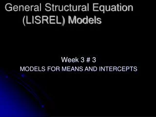
x y y y x y x x l21 l63 l21 l41 l42 l62 l73 l31 e e d e d d e e d d d d e q44 q33 q22 q11 q66 q77 q11 q33 q44 q55 q66 q55 q22 The general structural equation model j11 d1 x1 1 x1 y11 y22 y33 d2 x2 g11 j21 z1 z2 z3 j22 d3 x3 1 b21 b32 g12 j31 h1 x2 h2 h3 d4 x4 1 1 1 j32 g13 y5 y6 y7 d5 x5 1 y1 y2 y3 y4 e5 d6 e6 x3 x6 e1 e3 e2 e4 d7 x7 j33
x y y y x y x x l21 l63 l21 l41 l42 l62 l73 l31 e e d e d d e e d d d d e q44 q33 q22 q11 q66 q77 q11 q33 q44 q55 q66 q55 q22 The general structural equation model j11 d1 x1 1 x1 y11 y22 y33 d2 x2 g11 j21 z1 z2 z3 j22 d3 x3 1 b21 b32 g12 j31 h1 x2 h2 h3 d4 x4 1 1 1 j32 g13 y5 y6 y7 d5 x5 1 y1 y2 y3 y4 e5 d6 e6 x3 x6 e1 e3 e2 e4 d7 x7 j33
x y y y x y x x l21 l63 l21 l41 l42 l62 l73 l31 e e d e d d e e d d d d e q44 q33 q22 q11 q66 q77 q11 q33 q44 q55 q66 q55 q22 The general structural equation model j11 d1 x1 1 x1 y11 y22 y33 d2 x2 g11 j21 z1 z2 z3 j22 d3 x3 1 b21 b32 g12 j31 h1 x2 h2 h3 d4 x4 1 1 1 j32 g13 y5 y6 y7 d5 x5 1 y1 y2 y3 y4 e5 d6 e6 x3 x6 e1 e3 e2 e4 d7 x7 j33
x y y y x y x x l21 l63 l21 l41 l42 l62 l73 l31 e e d e d d e e d d d d e q44 q33 q22 q11 q66 q77 q11 q33 q44 q55 q66 q55 q22 The general structural equation model j11 d1 x1 1 x1 y11 y22 y33 d2 x2 g11 j21 z1 z2 z3 j22 d3 x3 1 b21 b32 g12 j31 h1 x2 h2 h3 d4 x4 1 1 1 j32 g13 y5 y6 y7 d5 x5 1 y1 y2 y3 y4 e5 d6 e6 x3 x6 e1 e3 e2 e4 d7 x7 j33
Why is it important to take into account measurement error? Consider the following model: Correction for attenuation:
Why is it important to take into account measurement error? (cont’d) The true effect of ξ on η is: The effect of x on y is:
Model identification • Necessary condition for identification • Two-step rule: • Measurement model • Latent variable model • Null B rule • Recursive rule • Rank condition • Empirical identification tests
SIMPLEX specification Title A general structural equation model (explaining coupon usage) Observed Variables id be1 be2 be3 be4 be5 be6 be7 aa1t1 aa2t1 aa3t1 aa4t1 bi1 bi2 bh1 Raw Data from File=d:\m554\eden2\sem.dat Latent Variables INCONV REWARDS ENCUMBR AACT BI BH Sample Size 250 Relationships be1 = 1*INCONV be2 = INCONV be3 = 1*REWARDS be4 = REWARDS be5 = 1*ENCUMBR be6 = ENCUMBR be7 = ENCUMBR aa1t1 = 1*AACT aa2t1 = AACT aa3t1 = AACT aa4t1 = AACT bi1 = 1*BI bi2 = BI bh1 = 1*BH AACT = INCONV REWARDS ENCUMBR BI = AACT BH = BI Set the Error Variance of bh1 to zero Options sc rs mi wp Path Diagram End of Problem
Goodness of Fit Statistics: Degrees of Freedom = 70 Minimum Fit Function Chi-Square = 93.63 (P = 0.031) Normal Theory Weighted Least Squares Chi-Square = 92.60 (P = 0.037) Estimated Non-centrality Parameter (NCP) = 22.60 90 Percent Confidence Interval for NCP = (1.60 ; 51.68) Minimum Fit Function Value = 0.38 Population Discrepancy Function Value (F0) = 0.091 90 Percent Confidence Interval for F0 = (0.0064 ; 0.21) Root Mean Square Error of Approximation (RMSEA) = 0.036 90 Percent Confidence Interval for RMSEA = (0.0096 ; 0.054) P-Value for Test of Close Fit (RMSEA < 0.05) = 0.89 Expected Cross-Validation Index (ECVI) = 0.65 90 Percent Confidence Interval for ECVI = (0.57 ; 0.77) ECVI for Saturated Model = 0.84 ECVI for Independence Model = 12.16 Chi-Square for Independence Model with 91 Degrees of Freedom = 2999.42 Independence AIC = 3027.42 Model AIC = 162.60 Saturated AIC = 210.00 Independence CAIC = 3090.72 Model CAIC = 320.85 Saturated CAIC = 684.75 Normed Fit Index (NFI) = 0.97 Non-Normed Fit Index (NNFI) = 0.99 Parsimony Normed Fit Index (PNFI) = 0.75 Comparative Fit Index (CFI) = 0.99 Incremental Fit Index (IFI) = 0.99 Relative Fit Index (RFI) = 0.96 Critical N (CN) = 268.08 Root Mean Square Residual (RMR) = 0.13 Standardized RMR = 0.049 Goodness of Fit Index (GFI) = 0.95 Adjusted Goodness of Fit Index (AGFI) = 0.92 Parsimony Goodness of Fit Index (PGFI) = 0.63
Measurement Equations aa1t1 = 1.00*AACT, Errorvar.= 0.68 , R2 = 0.63 (0.075) 9.06 aa2t1 = 1.04*AACT, Errorvar.= 0.44 , R2 = 0.74 (0.069) (0.058) 14.97 7.70 aa3t1 = 0.85*AACT, Errorvar.= 0.76 , R2 = 0.53 (0.070) (0.077) 12.14 9.82 aa4t1 = 1.10*AACT, Errorvar.= 0.59 , R2 = 0.71 (0.076) (0.072) 14.58 8.20 bi1 = 1.00*BI, Errorvar.= 0.97 , R2 = 0.75 (0.14) 7.04 bi2 = 1.09*BI, Errorvar.= 0.25 , R2 = 0.93 (0.058) (0.13) 18.91 1.95 bh1 = 1.00*BH,, R2 = 1.00
Measurement Equations • be1 = 1.00*INCONV, Errorvar.= 0.56 , R2 = 0.79 • (0.17) • 3.32 • be2 = 0.98*INCONV, Errorvar.= 0.61 , R2 = 0.77 • (0.087) (0.16) • 11.32 3.71 • be3 = 1.00*REWARDS, Errorvar.= 0.45 , R2 = 0.75 • (0.18) • 2.55 • be4 = 0.82*REWARDS, Errorvar.= 0.96 , R2 = 0.48 • (0.12) (0.15) • 6.89 6.63 • be5 = 1.00*ENCUMBR, Errorvar.= 2.78 , R2 = 0.24 • (0.28) • 9.97 • be6 = 1.73*ENCUMBR, Errorvar.= 1.85 , R2 = 0.59 • (0.27) (0.34) • 6.30 5.49 • be7 = 1.48*ENCUMBR, Errorvar.= 1.92 , R2 = 0.50 • (0.24) (0.28) • 6.30 6.87
Structural Equations AACT = - 0.28*INCONV + 0.44*REWARDS - 0.050*ENCUMBR, Errorvar.= 0.69 , R2 = 0.42 (0.058) (0.081) (0.097) (0.11) -4.77 5.42 -0.51 6.52 BI = 1.10*AACT, Errorvar.= 1.53 , R2 = 0.48 (0.11) (0.20) 10.04 7.73 BH = 0.49*BI, Errorvar.= 1.41 , R2 = 0.34 (0.049) (0.13) 10.10 10.78
Modification Indices for BETA AACT BI BH -------- -------- -------- AACT - - 11.05 1.52 BI - - - - 2.34 BH 2.34 - - - - Modification Indices for GAMMA INCONV REWARDS ENCUMBR -------- -------- -------- AACT - - - - - - BI 5.57 3.07 5.15 BH 1.61 12.67 2.78


![Structural Equation Model[l]ing (SEM)](https://cdn2.slideserve.com/5132235/slide1-dt.jpg)