Download
1 / 21
210 likes | 280 Vues
Computation on Parametric Curves. Yan-Bin Jia. Department of Computer Science Iowa State University Ames, IA 50011-1040, USA jia@cs.iastate.edu. Dec 16, 2002. Why Curved Objects?. Frequent subjects of maneuver (pen, mouse, cup, etc.).

E N D
Computation on Parametric Curves Yan-Bin Jia Department of Computer Science Iowa State University Ames, IA 50011-1040, USA jia@cs.iastate.edu Dec 16, 2002
Why Curved Objects? Frequent subjects of maneuver (pen, mouse, cup, etc.) Actions and mechanics are inherently continuous / differential and subject to local geometry of bodies Contact kinematics Dynamics Control Shape localization, recognition, reconstruction Not well studied compared to polygonal and polyhedral objects
Outline of the Talk 1. Constructing common tangents of two curves 2. Computing all pairs of antipodal points antipodal grasp Primitive used by other algorithms
Antipodal Grasp & Points Hong et al. 1990; Chen & Burdick 1992; Ponce et al. 1993; Blake & Taylor 1993 Grasping & Fixturing Salisbury & Roth 1983; Mishra et al. 1987; Nguyen 1988; Markenscoff et al. 1992; Trinkle 1992;Brost & Goldberg 1994; Bicchi 1995, Kumar & Bicchi 2000 Curve Processing Goodman 1991; Kriegman & Ponce 1991; Manocha & Canny 1992; Sakai 1999; Jia 2001 Computational Geometry Preparata & Hong 1977; Yao 1982; Chazelle et al. 1993; Matousek & Schwarzkopf 1996; Ramos 1997; Bespamyatnikh 1998 Previous Work
s a s b T(s ) T(s ) T(s ) T(s ) b b a a t t a b Common Tangent of Two Segments Assumptions for clarity (removable): i) Curvature everywhere positive or everywhere negative T ii) Opposite normals at corresponding endpoints S iii) Total curvatures (–, ) (and with equal absolute value) total curvature
How Many Common Tangents? Theorem Two segments satisfying conditions (i)—(iv) • have at most twocommon tangents incident on • points with opposite normals. b) are always on the same side of every common tangent or always on different sides.
Four Configurations (N, translation of tangents, etc) How to distinguish them?
t 0 s 0 s t 1 1 t t* s s* 2 2 Sequences { s } and { t } converge quadratically to s* and t*. k k An Iterative Procedure ( k 15, # low-level iterations 300) To find common tangencies with the same normal, reverse the normal vector field on one segment.
simple Inflection: = 0 but 0 Preprocessing I Step 1Compute all simple inflections. Step 2Split every segment whose total curvature [–, ]. > 0 > 0 < 0 < 0 Assumptions i)-iii) satisfied. Step 3 Shortening either or both segments
Application I – Convex Hull O(n) #inflections Van Dis & Jia 2002
limacon = 4 + 2.5 cos elliptic lemniscate 2 2 2 2 1/2 = (6 cos + 3 sin ) Application II – Antipodal Points closed cubic spline (10 pairs) = 3/(1+0.5 cos(3))
s* t* Antipodal Points Two pointswhose inward normals are i) collinear ii) pointing at each other. a simple close curve
Incomplete – not guaranteed to find one, not to mention all of them. Existing Methods formulation nonlinear programming + heuristics Inefficient – many initial estimates often needed. Why not exploit global & local (differential) geometry together?
t Locally, define opposite points by N(t ) N(s) + N(t) = 0 N(s) : antipodal angle Assumption iv) Normals at opposite points (s, t) point towards each other. s Antipodal Angle s and t are antipodal if and only if (s) = 0. t* r(s) s* simple antipodal pointss* and t* if (s*) = 0 but (s*) 0.
uniquepair of antipodal points if (s )< 0 and (s )> 0. a b s s b a (s ) (s ) a b s* Bisection over [s , s ]. a b t* t t a b Opposite Angle Sign at Endpoints antipodal angleincreases monotonicallyas s increases. no antipodal points otherwise. Both segments are concave. S T
t t 1 2 t = 0 0 1 t t b a monotone sequences s ,s , … t , t , … 0 1 s s a a s = s 0 2 s 1 Same Angle Sign at Endpoints Marching I (convex-convex) t* If exist, linear convergence to the closest pair. s* Otherwise, termination at the other endpoints.
The ray of N(t ) or N(t ) must intersect segment S a b t t b a s s b a monotone sequences: s ,s , … 0 1 t , t , … t 0 1 t = t* 1 0 t 2 s* s 2 s 1 s = 0 Cont’d Marching II (convex-concave) Same convergence result
s* 2 t* s* 1 1 Recursion tree: s* , t* 1 1 t* Case 1 (march) 2 march s* , t* bisection Case 2 (bisection) 2 2 Case 1 Case 1 Recursively Finding All pairs
s s b a t b t a Preprocessing II a pair of normals pointing away from each other Steps 1, 2, 3 Step 4Compute common tangent lines
running time is tight 2 Efficiency – O(n + m)two-level calls of numerical primitives Conclusion Design of algorithms for curve computing Dissecting the curve into monotone segments (preprocessing of global geometry) Interleaving marching with numerical bisection (exploiting of local geometry) Provable convergence rates (depending on curvatures) Completeness – up to numerical resolution #inflections #antipodal pairs
Extension Algebraic Curves 2-D Surfaces Optimization along Curves, Surfaces