Multi-criteria Landuse Planning

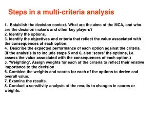
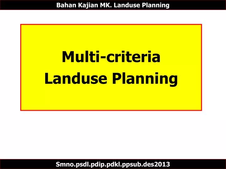
BahanKajian MK. Landuse Planning Multi-criteria Landuse Planning Smno.psdl.pdip.pdkl.ppsub.des2013

Pendahuluan • Land is a scarce resource • essential to make best possible use • identifying suitability for: • agriculture • forestry • recreation • housing • etc.

Sieve mapping • Early methods • Ian McHarg (1969) Design with Nature • tracing paper overlays • landscape architecture and facilities location • Bibby & Mackney (1969) Land use capability classification • tracing paper overlays • optimal agricultural land use mapping

GIS approaches Sieve mapping using: • polygon overlay (Boolean logic) • cartographic modelling • Example uses: • nuclear waste disposal site location • highway routing • land suitability mapping • etc.

Sieve mapping / boolean overlay The easiest way to do sieve mapping to use Boolean logic to find combinations of layers that are defined by using logical operators: AND for intersection, OR for union, and NOT for exclusion of areas (Jones, 1997). In this approach, the criterion is either true or false. Areas are designated by a simple binary number, 1, including, or 0, excluding them from being suitable for consideration (Eastman, 1999).

Boolean example Within 500m from Shepshed Within 450m from roads Slope between 0 and 2.5% Land grade III Suitable land, min 2.5 ha

Definitions • Decision: a choice between alternatives • Decision frame: the set of all possible alternatives • [ Parks Forestry ] • Candidate set: the set of all locations [pixels] that are being considered • [ all Crown lands ] • Decision set: the areas assigned to a decision (one alternative) • [ all pixels identified as Park ]

Definitions • Criterion: some basis for a decision. Two main classes: • Factors: enhance or detract from the suitability of a land use alternative (OIR) [e.g., distance from a road] • Constraints: limit the alternatives (N) [e.g., crown/private lands] [boolean] • Can be a continuum from crisp decision rules (constraints) to fuzzy decision rules (factors) • Goal or target: some characteristic that the solution must possess (a positive constraint) • E.g., 12% of the land base identified as park

Definitions • Decision rule: the procedure by which criteria are combined to make a decision. Can be: • Functions: numerical, exact decision rules • Heuristics: approximate procedures for finding solutions that are ‘good enough’ • Objective: the measure by which the decision rule operates (e.g., identify potential parks) • Evaluation: the actual process of applying the decision rule

Kinds of evaluations • Single-criterion evaluation (e.g., do I have enough money to see a movie?) • Multi-criteria evaluation: to meet one objective, several criteria must be considered (e.g., do I have enough $ to see a movie, do I want to see an action flick or a horror movie, which theatre is closest?) • Multi-objective evaluations: • Complementary objectives: non-conflicting objectives (e.g., extensive grazing and recreational hiking) • Conflicting objectives: both cannot exist at the same place, same time (e.g., ecological reserves and timber licenses)

Multi-criteria evaluation • Basic MCE theory: • “Investigate a number of choice possibilities in the light of multiple criteria and conflicting objectives” (Voogd, 1983) • Generate rankings of choice alternatives • Two basic methodologies: • Boolean overlays (polygon-based methods) [A] • Weighted linear combinations (WLC) (raster-based methods) [B] B A

Multi-criteria evaluation Multicriteriaanalysis appeared in the 1960s as a decision-making tool. It is used to make a comparative assessment of alternative projects or heterogeneous measures. With this technique, several criteria can be taken into account simultaneously in a complex situation. The method is designed to help decision-makers to integrate the different options, reflecting the opinions of the actors concerned, into a prospective or retrospective framework. Participation of the decision-makers in the process is a central part of the approach. The results are usually directed at providing operational advice or recommendations for future activities.

Multi-criteria evaluation • Multicriteria evaluation be organised with a view to producing a single synthetic conclusion at the end of the evaluation or, on the contrary, with a view to producing conclusions adapted to the preferences and priorities of several different partners. • Multi-criteria analysis is a tool for comparison in which several points of view are taken into account, and therefore is particularly useful during the formulation of a judgement on complex problems. The analysis can be used with contradictory judgement criteria (for example, comparing jobs with the environment) or when a choice between the criteria is difficult.

MCE • Non-monetary decision making tool • Developed for complex problems,where uncertainty can arise if a logical, well-structured decision-making process is not followed • Reaching consensus in a (multidisciplinary) group is difficult to achieve.

Teknik-Teknik MCE • Many techniques (decision rules) • Most developed for evaluating small problem sets (few criteria, limited candidate sets) • Some are suitable for large (GIS) matrices • layers = criteria • cells or polygons = choice alternatives • Incorporation of levels of importance (weights – WLC methods) • Incorporation of constraints (binary maps)

MCE – pros and cons Cons: • Dynamic problems strongly simplified into a linear model • Static, lacks the time dimension • Controversial method – too subjective? Pros: • Gives a structured and traceable analysis • Possibility to use different evaluation factors makes it a good tool for discussion • Copes with large amounts of information • It works!

MCE – pros and cons • MCE is not perfect…“quick and dirty”-option, unattractive for “real analysts” • … but what are the alternatives?- system dynamics modelling impossible for huge socio-technical problems - BOGSATT is not satisfactory (Bunch of Old Guys/Gals Sitting Around a Table Talking) • MCE is good for complex spatial problems • Emphasis on selecting good criteria, data collection and sensitivity analysis

Prinsip-prinsip MCE • Methodology • Determine criteria (factors / constraints) to be included • Standardization (normalization) of factors / criterion scores • Determining the weights for each factor • Evaluation using MCE algorithms • Sensitivity analysis of results

MenentukanKriteria • Oversimplification of the decision problem could lead to too few criteria being used • Using a large number of criteria reduces the influence of any one criteria • They should be comprehensive, measurable, operational, non-redundant, and minimal • Often proxies must be used since the criteria of interest may not be determinable (e.g., % slope is used to represent slope stability) • A multistep, iterative process that considers the literature, analytical studies and, possibly, opinions

FaktorNormalisasi Good: 255 255 Output Output Poor: 0 0 low high low high Input Input • Standardization of the criteria to a common scale (commensuration) • Need to compare apples to apples, not apples to oranges to walnuts. For example: • Distance from a road (km) • Slope (%) • Wind speed • Consider • Range (convert all to a common range) • Meaning (which end of the scale = good)

Fuzzy membership functions Used to standardize the criterion scores Linguistic concepts are inherently fuzzy (hot/cold; short/tall)

Menentukan Pembobot • By normalizing the factors we make the choice of the weights an explicit process. • A decision is the result of a comparison of one or more alternatives with respect to one or more criteria that we consider relevant for the task at hand. Among the relevant criteria we consider some as more important and some as less important; this is equivalent to assigning weights to the criterion according to their relative importance.

Menentukan Pembobot Multiple criteria typically have varying importance. To illustrate this, each criterion can be assigned a specific weight that reflects it importance relative to other criteria under consideration. The weight value is not only dependent the importance of any criterion, it is also dependent on the possible range of the criterion values. A criterion with variability will contribute more to the outcome of the alternative and should consequently be regarded as more important than criteria with no or little changes in their range.

MenentukanPembobot • Weights are usually normalised to sum up to 1, so that in a set of weights (w1, w2, ., wn) =1. • There are several methods for deriving weights, among them (Malczewski, 1999): • Ranking • Rating • Pairwise Comparison (AHP) • Trade-off • The simplest way is straight ranking (in order of preference: 1=most important, 2=second most important, etc.). Then the ranking is converted into numerical weights on a scale from 0 to 1, so that they sum up to 1.

AHP: Analytical hierarchy process One of the more commonly-used methods to calculate the weights.

AHP: Analytical hierarchy process • IDRISI features a weight routine to calculate weights, based on the pairwise comparison method, developed by Saaty (1980). A matrix is constructed, where each criterion is compared with the other criteria, relative to its importance, on a scale from 1 to 9. Then, a weight estimate is calculated and used to derive a consistency ratio (CR) of the pairwise comparisons. • If CR > 0.10, then some pairwise values need to be reconsidered and the process is repeated till the desired value of CR < 0.10 is reached.

MCE Algorithms • The most commonly used decision rule is the weighted linear combination • where: • S is the composite suitability score • x – factor scores (cells) • w – weights assigned to each factor • c – constraints (or boolean factors) • ∑ -- sum of weighted factors • ∏ -- product of constraints (1-suitable, 0-unsuitable) S = ∑wixi x ∏cj

MCE • A major difference between boolean (sieve methods) and MCE is that for boolean [and] methods every condition must be met before an area is included in the decision set. There is no distinction between those areas that “fully’ meet the criteria and those that are at the “edges” of the criteria. • There is also no room for weighting the factors differentially.

Map 1 Map 2 Map 3 Map 4 Standardise Evaluation matrix User weights MCE routine Output Example: weighted linear summation

Sensitivity analysis • Choice for criteria (e.g., why included?) • Reliability data • Choice for weighing factors is subjective • Will the overall solution change if you use other weighing factors? • How stable is the final conclusion? • sensitivity analysis: vary the scores / weights of the factors to determine the sensitivity of the solution to minor changes

Sensitivity analysis • Only addresses one of the sources of uncertainty involved in making a decision (i.e., the validity of the information used) • A second source of uncertainty concerns future events that might lead to differentially preferred outcomes for a particular decision alternative. • Decision rule uncertainty should also be considered (? MCE itself)

Vibriocholerae • Untreated: death within 24h from loss of fluid • Transmission: ingest contaminated material • Treatment: fluid replacement and antibiotics • Origins in the Orient • Now endemic in many places

Geosphere Biosphere (plants&animals) Atmosphere (air) V. cholerae Lithosphere (soil) Hydrosphere (water) The complex nature of cholera

Transmitted to humans: • Ingestion of an infectious dose of V. cholerae(critical threshold value of 106 cells) • Socio-cultural-economic vulnerability factors Transmission to humans Zooplankton: • V. cholerae associates with zooplankton for survival, multiplication & transmission purposes Zooplankton: copepods & other crustaceans (fresh & saltwater systems) Algae: • Promote survival of V. cholerae • Provide indirectly favourable conditions for growth and maybe expression of virulence • Provide food for zooplankton Phytoplankton & Aquatic plants Temperature, pH Fe+, salinity sunlight Abiotic conditions: • Favour growth of V. cholerae and/or • expression of virulence Hierarchical approach

Inputs Literature survey and expert workshops to: • Determine possible contributing factors to a cholera outbreak Simulation model to: • Provide some of the input into the expert system • Simulate the relative importance of different variables Expert system to: • Capture the knowledge and data • Establish the high-level structure and flow of the integrated model GIS and fuzzy logic to implement model thus defined Outputs • Possible cholera outbreak location and date

Variable Range Optimal value Occurrence of cholera in the past Poor indication of epidemic reservoir Average rainfall (mm/month) > 600mm Mean maximum daily surface temperature (C/day) 30-38C 37 (<15C reduces growth and survival rates significantly) Number of consecutive ‘hot’ months overlapping with the rainy season 1-4 >1 month Salinity for growth purposes (total salts, %). 0-45 Values between 5-25% considered to be optimal Salinity for expression of toxigenity (total salts, %) (Häse and Barquera, 2001). 0.05-2.5 Values between 2-2.5% considered to be optimal pH 8-8.6 8.2 (< 4.6 with low temperatures reduce growth and survival rates significantly) Fe+ (soluble and/or insoluble form) Must be present (moderate amounts) Low<0.1 Moderate=0.1 to 0.5 High>0.5 Presence of phytoplankton and algae Similar growth & survival factors. Photosynthesis also increases pH. Presence of zooplankton The simple presence of crustacean copepods enhances the survival of V. cholerae Dissolved Oxygen daily cycles for every month of the year (mg/l) Daily fluctuations provide a preliminary indication of algal blooms Oxidation-Reduction Potential daily cycles for every month of the year Model variables

MCE @ Shepshed 100m < Shepshed <1000m Between 50m and 600m to roads Slope between 1 and 5% Land grade III and grade IV Varying suitability, min 2.5 ha Bright areas have highest suitability

Comparison of results The Boolean constrains leave no room for prioritisation, all suitable areas are of equal value, regardless of their position in reference to their factors. Minimal fuzzy membership: the minimum suitability value from each factor at that location is chosen from as the "worst case" suitability. This can result in larger areas, with highly suitable areas. Probabilistic fuzzy intersection: fewer suitable areas than the minimal fuzzy operation. This is due to the fact that this effectively is a multiplication. Multiplying suitability factors of 0.9 and 0.9 at one location yields an overall suitability of 0.81, whereas the fuzzy approach results in 0.9. Thus, it can be argued that the probabilistic operation is counterproductive when using fuzzy variables (Fisher, 1994). When using suitability values larger than 1 this does of course not occur. Weighted Overlay: produces many more areas. This shows all possible solutions, regardless whether all factors apply or not, as long as at least one factor is valid for that area. This is so, because even if one factor is null, the other factors still sum up to a value. This also shows areas that are outside of the initial constraints. http://www.husdal.com/blog/2002/09/how-to-use-idri.html

Spatial Analytical Hierarchy Process • Wind farm siting • Find the best wind farm sites based on siting factors • Alternatives • Location—infinite • Divide the space into squares/cells (200m * 200m) • Evaluate each cell based on the siting factors

Preliminary Siting Factors • Accessibility to roads • Distance to primary roads • Distance to secondary roads • Distance to rural roads • Accessibility to transmission lines • Distance to 100K lines • Distance to 250K lines • Distance to above250K lines • Wind power (or wind speed) • Visibility • Viewshed size • # of people in viewshed

Siting Steps (MCE) • Factor generation • Distance calculation • Visibility calculation • Factor standardization (0 – 100) • Each factor is a map layer • Factor weights determination by AHP • Final score • Weighted combination of factors • Exclusion areas

AHP

Factor Layers

Wind Turbine Viewshed Size • Red—505km2 • Greed--805km2 • Blue--365km2 • Software tool developed to calculate viewshed size for each cell

Visibility Factor—Viewshed Size • Computational expensive • About 700,000 cells • Each cell requires 10 seconds • About 76 days • Parallel computing • 12 computers • Each computer runs two counties • About 55000 cells • 6 days • Succeed with 3000 cells but failed with 55,000 cells

2000 census block data Visibility Factor--# of People in Viewshed

Final Score Layer

Candidate Sites

Constraints (binary)

Sites

Multi-criteria Landuse Planning