Maxwell’s Equations

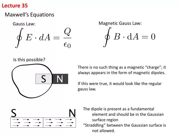
1. Lecture 35 Maxwell’s Equations Magnetic Gauss Law: Gauss Law: Is this possible? There is no such thing as a magnetic “charge”; it always appears in the form of magnetic dipoles. If this were true, it would look like the regular gauss law. The dipole is present as afundamental element and should be in the Gaussian surface region “Straddling” between the Gaussian surface is not allowed.

2. Maxwell’s Equations – continued... Ampere’s Law Current running through the surface where the rim of the surface = path (think of the surface as a soap bubble filament) Mathematically, the film doesn’t need to be flat , Charge build-up on the plate generates an electric flux Responsible for piercing the surface defined by the rim (Virtual current, or the displacement current ID, to be added to “I” in Amp-Maxwell Law) (For partial piercing, refer to Fig(mi) 24.5)

3. Discussion of Ch24.Hw1.001 Set-up: , increasing Apply Ampere-Maxwell Law: P (2) (1) Caution, check contributions of: Exercise: Check various cases: Clicker 1: correct

4. One Dimensional EM Pulse We use the following example used by Professor Feynman to illustrate some of the properties of EM pulse. The geometry of the setup is shown in fig 35.2 and fig 35.3 A warm up. There is the presence of a current sheet at x = 0 in the yz-plane. If the current I is constant, it generates a familiar B pattern shown in fig 35.4 For x > 0, B-lines are pointing in the –z direction. For x < 0, B lines are in the +z direction. Now we proceed to discuss the generation of 1D-EM pulse in steps.

5. Step 1: Instead of having a steady current, we turn on the current at t = 0. Here there is no B-pattern before t = 0. The pattern immediately setups when t > 0. First, the B pattern is created in the proximity of x = 0. As t increases there is the spread both in x > 0 and in x < 0 direction with a speed of v. The goal of this exercise is to use fig 35.2 and fig 35.3 determine v. Step 2: In fig 35.21 and fig 35.2b define the closed path 12341. The loop is in the xy plane at some z value. We view how the flux grows within the window. As shown in Fig 35.2b, the B-flux in the window increases, as the flux expands to the right. The flux is defined by

6. Lenz rule states as the B flux into the window increases, there must be Bind, the induced B, pointing out of the loop, which opposes the increase of the ingoing flux. Bind is caused by CCW emf induced. The Faraday’s Law using the closed path 12341 gives: Step 3: Eind in step 2 is the E field of the EM pulse discussed in Sec. 24.2 in the text. One sees that E x B for the present case is along to the right. We proceed to shown that Ampere-Maxwell law (AM-law) leads to an additional relationship between E and B which will enable us to determine v. (1)

7. Consider the AM-loop 12561 shown in (a) and (b) of Fig35.3. Fig35.3a shows the front view where the loop is at the top. Fig35.3b shows the top view of the loop. AM-law states: or This combined with (1) E = Bv leads to Thus EM pulse travels in free space with an universal speed, the speed of light.

8. Recap: Propagation of EM waves: 1. gives the direction of propagation , 2. Universal Speed (in a vacuum) All light is an EM wave, and travels with the same speed 3. Reflection: c is the speed of the “wavefront” Field has a boundary. This boundary travels with v = c in vacuum. The wave shape is initiated by the t-dependence of the source. For sinusoidal current: The squares are rounded off