Download
1 / 1
10 likes | 91 Vues
Modeling the Gas-Grain Plume of Enceladus. θ sp. S. K. Yeoh , T. A. Chapman, D. B. Goldstein, P. L. Varghese, L. M. Trafton The University of Texas at Austin; E-mail: skyeoh@utexas.edu. Credit: NASA/JPL. Credit: NASA/JPL. Introduction. Far-field Results vs. Cassini INMS Data. Vent.

E N D
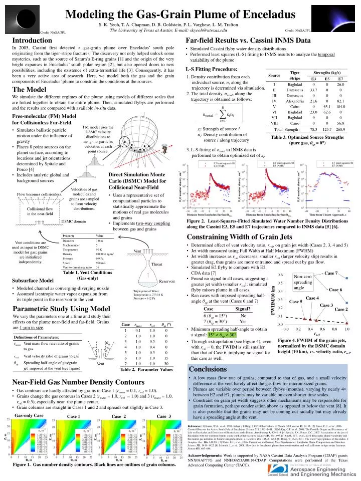
Modeling the Gas-Grain Plume of Enceladus θsp S. K. Yeoh, T. A. Chapman, D. B. Goldstein, P. L. Varghese, L. M. Trafton The University of Texas at Austin; E-mail: skyeoh@utexas.edu Credit: NASA/JPL Credit: NASA/JPL Introduction Far-field Results vs. Cassini INMS Data Vent In 2005, Cassini first detected a gas-grain plume over Enceladus’ south pole originating from the tiger-stripe fractures. The discovery not only helped unlock some mysteries, such as the source of Saturn’s E-ring grains [1] and the origin of the very bright expanses in Enceladus’ south polar region [2], but also opened doors to new possibilities, including the existence of extra-terrestrial life [3]. Consequently, it has been a very active area of research. Here, we model both the gas and the grain components of Enceladus’ plume to constrain the conditions at the sources. • Simulated Cassini flyby water density distributions • Performed least squares (L-S) fitting to INMS results to analyze the temporal variability of the plume L-S Fitting Procedure: 1. Density contribution from each individual source, n, along the trajectory is determined via simulation. 2. The total density, ntotal, along the trajectory is obtained as follows: 3. L-S fitting of ntotal to INMS data is performed to obtain optimized set of si. The Model We simulate the different regimes of the plume using models of different scales that are linked together to obtain the entire plume. Then, simulated flybys are performed and the results are compared with available in-situ data. Vent Throat FM model uses the DSMC velocity distributions to assign its particles velocities at each point source. si: Strength of source i ni: Density contribution of source i along trajectory Table 3. Optimized Source Strengths (pure gas, θsp = 0) Reservoir Free-molecular (FM) Model for Collisionless Far-Field • Simulates ballistic particle motion under the influence of gravity • Places 8 point sources on the planet surface, according to locations and jet orientations determined by Spitale and Porco [4] • Includes analytic global and background sources Velocities of gas molecules and grains are sampled to form velocity distributions. Direct Simulation Monte Carlo (DSMC) Model for Collisional Near-Field Figure 2. Least-Squares-Fitted Simulated Water Number Density Distributions along the Cassini E3, E5 and E7 trajectories compared to INMS data [5] [6]. • Uses a representative set of computational particles to statistically approximate the motions of real gas molecules and grains • Implements two-way coupling between gas and grains Flow becomes collisionless. Subsurface Model • Modeled channel as converging-diverging nozzle • Assumed isentropic water vapor expansion from its triple point in the reservoir to the vent Constraining Width of Grain Jets Collisional flow in the near-field Vent conditions are used as input to DSMC model for gas; grains are initialized independently. • Determined effect of vent velocity ratio, rvel, on grain jet width (Cases 2, 3, 4 and 5) • Jet width measured using Full Width at Half Maximum (FWHM) • Jet width increases as rveldecreases; smaller rvel (larger velocity slip) results in greater drag, thus grains are more entrained and spread out by gas flow. DSMC domain • Simulated E2 flyby to compare with E2 CDA data [7] • Found no signal in all cases, suggesting a greater jet width (smaller rvel); simulated flyby misses plume in all cases. • Ran cases with imposed spreading half-angle θsp at the vent (Cases 6 and 7) • Minimum spreading half-angle to obtain a signal: 15 < θsp < 30 Table 1. Vent Conditions (Gas-only) Case 7 Triple point of Water: Temperature = 273.16 K Pressure = 612 Pa Non-zero spreading angle Parametric Study Using Model Case 6 We vary the parameters one at a time and study their effects on the plume near-field and far-field. Grains are 1-µm in size. Case 4 Case 5 Case 3 Case 2 Figure 4. FWHM of the grain jets, normalized by the DSMC domain height (10 km), vs. velocity ratio, rvel. • Through extrapolation (see Figure 4), even with rvel= 0, the FWHM is still smaller than that of Case 6, implying no signal for this case as well. Conclusions Table 2. Parameter Values • A low mass flow rate of grains, compared to that of gas, and a small velocity difference at the vent barely affect the gas flow for micron-sized grains. • Plumes are variable over period between flybys (months), varying by nearly 4× between E2 and E7; plumes may be variable on even shorter time scales. • Constraint on grain jet width suggests other mechanisms may be responsible for grain formation, perhaps condensation above as opposed to below the vent [8]. It is also possible that the grains may not be coming out radially but may already have a spreading angle at the vent. Near-Field Gas Number Density Contours Gas-only Case • Gas contours are hardly affected by grains in Case 1 (rmass = 0.1, rvel = 1.0). • Grains change the gas contours in Cases 2 (rmass = 1.0, rvel = 1.0) and 3 (rmass = 1.0, rvel = 0.5), especially near the plume center. • Grain columns are straight in Cases 1 and 2 and spreads out slightly in Case 3. Case 1 Case 3 Case 2 References:[1] Baum, W.A., et al., 1981. Saturn’s E Ring: I. CCD Observations of March 1980. Icarus47, 84–96. [2]Porco, C.C., et al., 2006. Cassini Observes the Active South Pole of Enceladus. Science311, 1393–1401.[3] McKay, C.P., et al., 2008. The Possible Origin and Persistence of Life on Enceladus and Detection of Biomarkers in the Plume. Astrobiology8, 909–919.[4] Spitale, J.N., Porco, C.C., 2007. Association of the jets of Enceladus with the warmest regions on its south-polar fractures. Nature449, 695–697. [5] Smith, H.T., et al., 2010. Enceladus plume variability and the neutral gas densities in Saturn’s magnetosphere. J. Geophys. Res.115, A10252. [6] Dong, Y., et al., 2011. The water vapor plumes of Enceladus. J. Geophys. Res. 116, A10204. [7] Waite, J.H., et al., 2006. Cassini Ion and Neutral Mass Spectrometer: Enceladus Plume Composition and Structure. Science311, 1419–1422. [8] Schmidt, J., et al., 2008. Slow dust in Enceladus’ plume from condensation and wall collisions in tiger stripe fractures. Nature451, 685–688. Acknowledgements:Work is supported byNASA Cassini Data Analysis Program (CDAP) grants NNX08AP77G and NNH09ZDA001N-CDAP. Computations were performed at theTexas Advanced Computing Center (TACC). Figure 1. Gas number density contours. Black lines are outlines of grain columns.