Download
1 / 42
420 likes | 516 Vues
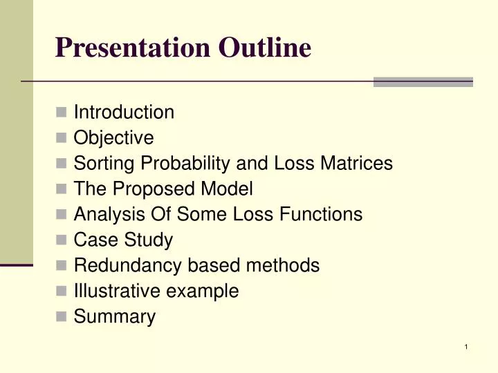
Presentation Outline. Introduction Objective Sorting Probability and Loss Matrices The Proposed Model Analysis Of Some Loss Functions Case Study Redundancy based methods Illustrative example Summary. Introduction. Accuracy and Precision Types of data Binary Situation.

E N D
Presentation Outline • Introduction • Objective • Sorting Probability and Loss Matrices • The Proposed Model • Analysis Of Some Loss Functions • Case Study • Redundancy based methods • Illustrative example • Summary
Introduction • Accuracy and Precision • Types of data • Binary Situation
A. Accuracy and Precision. Accuracy The closeness of agreement between the result of measurement and the true (reference) value of the product being sorted. Precision Estimate of both the variation in repeated measurements obtained under the same conditions (Repeatability) and the variation of repeated measurements obtained under different conditions (Reproducibility).
B. Two types of data characterizing products or processes Variables (results of measurement, Interval or Ratio Scales) Attributes(results of testing, Nominal or Ordinal Scales ).
Four types of data • The four levels were proposed by Stanley Smith Stevens in his 1946 article.Different mathematical operations on variables are possible, depending on the level at which a variable is measured.
Categorical Variables 1. Nominal scale: • gender, • race, • religious affiliation, • the number of a bus. Possible operations:
Categorical Variables(cont.) 2.Ordinal scale : • results of internet page rank, • alphabetic order, • Mohs hardness scale (10 levels from talc to diamond) • customer satisfaction grade , • quality sort, • customer importance (QFD) • vendor’s priority, • severity of failure or RPN (FMECA), • the power of linkage (QFD) Possible operations:
Numerical data. 3. Interval scale: • temperature in Celsius or Fahrenheit scale , • object coordinate, • electric potential. Possible operations:
Numerical data (cont.) 4. Ratio scale: • most physical quantities, such as mass, or energy, • temperature, when it is measured in kelvins, • amount of children in family, • age. Possible operations:
C. The sortingprobability matrixfor the binary situation Accuracy is characterized by: • Type I Errors (non-defective is reported as defective) –alfa risk • Type II Errors (defective is reported as non-defective) –beta risk
The sortingprobability matrixfor the binary situation (cont.)
Objective Developing a new statistical procedure for evaluating the accuracy and effectiveness of measurement systems applicable to Attribute Data based on the Taguchi approach.
Sorting Probability Matrix • The sorting matrix is an 'm by m' matrix. • Its components Pi,j are the conditional probabilities that an item will be classified as quality level j, given its quality level is i. • A stochastic matrix:
Four Interesting Sorting Matrices • (a) The most exact sorting: • (b) The uniform sorting: (designated as MDS: most disordered sorting): • (c) The “worst case” sorting. For example, if m = 4:
Four Interesting Sorting Matrices (cont.) (d) Absence of any sorting .For example, if m = 2:
Loss Matrix Definition Let Lij - be the loss incurred by classifying sort i as sort j.
The Proposed Model Expected Loss Definition: Effectiveness Measure:
Analysis Of Some Loss Functions • Equal loss: • Quadratic loss: • Entropy loss: • Linear loss:
Equal loss If there is no preliminary information about pi
Equal loss (Cont.) If any preliminary information about pi is available:
Quadratic Loss For ordinal data, the total accuracy of the rating could be defined as the expected value of Lij.
Quadratic Loss (Cont.) If there is no preliminary information about pi: If there is any preliminary information about pi:
Entropy loss If level i is systematically related to level j (Pij=1), there is no “entropy loss”. The above loss function leads us directly to Eff = Theil’s uncertainty index.
Linear Loss Could be useful for bias evaluation: This measure characterizes the dominant tendency [over grading, if Bias > 0 or under grading, if Bias < 0 ]
Case Study (nectarines sorting) Type 1- 0.860, Type 2 - 0.098 , Type 3 -0.042
Effectiveness Evaluations According to proposed approach: Eff = 80% Compare the above to the measures of effectiveness for different loss functions : • Equal loss: 74%. • Taguchi loss: 87%. • Disorder entropy loss: 62% • Linear penalty function:79% • Traditional kappa measure : 79% . It can be seen that the effectiveness estimate strongly depends on the loss metric model.
Case A: Two Independent Repeated Ratings • Real improvement may be obtained if, in the case of disagreement, the final decision is made in favor of the inferior sort (one rater can see a defect, which the other has not detected). • Usually, the loss that results from overrating is greater than the loss due to underrating, thus such a redistribution of probabilities seems to be legitimate. Nevertheless, to verify improvement in sorting effectiveness, we need a new expected loss calculation.
Case B: Three Repeated Ratings We add a third rater only if the first two raters do not agree. For most industrial applications this means that a product is passed through a scrupulous laboratory inspection or, for the purpose of our analysis, through an MRB board. The decision could be considered as an etalon measurement. The probability of correct decisions increases, and the probability of wrong decisions, decreases.
Conclusions To decide whether a double or triple rating procedure is expedient the total expenditures have to be compared
Case C: A Hierarchical ClassificationSystem • The classification procedure is built on more than one level. • To characterize such a hierarchical classification system G can be utilized as a “pure” indicator of the classification system’s inexactness. • Usually, the cost of classification (COC) has an inverse relationship to the amount ofG. In contrast to the COC, the expected loss usually decreases, as the exactness of the judgment improves.
Optimization of HCS If one decides to pass the hierarchical classification subsystem from the lower level (1) up to the Klevel, the total expenditure can be optimized by looking for the best level minimizing it .
A CASE STUDY AND ILLUSTRATIVE EXAMPLE The proportions of the sort types were: Type 1- 0.53, Type 2 - 0.27 and Type 3 - 0.20. The same loss matrix was considered. From an R&R study, executed in relation to two independent raters’ results, the joint probability matrices were estimated.
Summary • The proposed procedure for evaluation of product quality classifiers takes into account some a priori knowledge about the incoming product, errors of sorting and losses due to under/over graduation.
Summary (Cont.1) • The appropriate choice of the loss function (matrix) provides the opportunity to fit quality sorting process model to the real situation. • The effectiveness of quality classifying can be improved by different redundancy based methods. However, the advantages of redundancy based methods are not unequivocal, as is the case in the usual measurement processes, and corresponding calculations according to the technique being used are required.
Summary (Cont.2) • The conclusion concerning the selection of the preferred case depends on the losses due to misclassification, as well as on the incoming quality sort distribution. • Possible applications of the proposed approach are not limited only to quality sorting. The approach can be extended to other QA processes concerned with classification