Download
1 / 32
360 likes | 619 Vues
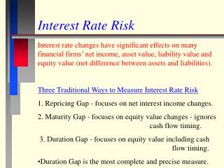
CHAPTER 13 Measurement of Interest-Rate Risk for ALM. What is in this Chapter? INTRODUCTION RATE-SHIFT SCENARIOS SIMULATION METHODS . INTRODUCTION. The purposes of measuring ALM interest-rate risk establish the amount of economic capital to be held against such risks

E N D
CHAPTER 13Measurement of Interest-Rate Risk for ALM What is in this Chapter? INTRODUCTION RATE-SHIFT SCENARIOS SIMULATION METHODS
INTRODUCTION • The purposes of measuring ALM interest-rate risk • establish the amount of economic capital to be held against such risks • How to reduce the risks by buying or selling interest-rate-sensitive instruments • Although ALM risk is a form of market risk, it cannot be effectively measured using the trading- VaR framework
This VaR framework is inadequate for two reasons. • First, the ALM cash flows are complex functions of customer behavior. • Second, interest-rate movements over long time horizons are not well modeled by the simple assumptions used for VaR.
INTRODUCTION • Banks use three alternative approaches to measure ALM interest-rate risk, as listed below: • Gap reports (缺口報告) • Rate-shift scenarios • Simulation methods similar to Monte Carlo VaR
GAP REPORTS • The "gap“ is the difference between the cash flows from assets and liabilities • Gap reports are useful because they are relatively easy to create • This measure is only approximate because gap reports do not include information on the way customers exercise their implicit options in different interest environments • There are three types of gap reports: contractual maturity, repricing frequency and effective maturity
Contractual-Maturity Gap Reports • A contractual-maturity gap report indicates when cash flows are contracted to be paid for liabilities, it is the time when payments would be due from the bank, assuming that customers did not roll over their accounts. • For example, the contractual maturity for checking accounts is zero because customers have the right to withdraw their funds immediately.
Contractual-Maturity Gap Reports • The contractual maturity for a portfolio of three-month certificates of deposit would (on average) be a ladder of equal payments from zero to three months. • The contractual maturity for assets may or may not include assumptions about prepayments. • In the most simple reports, all payments are assumed to occur on the last day of the contract
Repricing Gap Reports • Repricing Gap Reports • Repricing refers to when and how the interest payments will be reset
Effective-Maturity Gap Reports • Although the repricing report includes the effect of interest-rate changes, it does not include the effects of customer behavior. • This additional interest-rate risk is captured by showing the effective maturity. • For example, the effective maturity for a mortgage includes the expected prepayments, and may include an adjustment to approximate the risk arising from the response of prepayments to changes in interest rates.
Effective-Maturity Gap Reports • Gap reports give an intuitive view of the balance sheet, but they represent the instruments as fixed cash flows, and therefore do not allow any analysis of the nonlinearity of the value of the customers' options. • To capture this nonlinear risk requires approaches that allow cash flows to change as a function of rates.
Estimating Economic Capital based on Gap Reports • For this analysis, we made several significant assumptions: • We assumed that value changes linearly with rate changes • We also assumed that the duration would be constant over the whole year (prepayment and withdraw behavior?)
Estimating Economic Capital based on Gap Reports • Finally, we assumed that annual rate changes were Normally distributed. • These assumptions could easily create a 20% to 50% error in the estimation of capital • The methods that do not require so many assumptions (please refer to Page 194 to 195)
RATE-SHIFT SCENARIOS • Rate-shift scenarios attempt to capture the nonlinear behavior of customers. • A common scenario test is to shift all rates up by 1 %. • After shifting the rates, the cash flows are changed according to the behavior expected in the new environment
RATE-SHIFT SCENARIOS • For example, mortgage prepayments may increase, some of the checking and savings accounts may be withdrawn, and the prime rate may increase after a delay. • The NPV of this new set of cash flows is then calculated using the new rates.
RATE-SHIFT SCENARIOS • As an example, let us consider a bank with $90 million in savings accounts and $100 million in fixed-rate mortgages. • Assume that the current interbank rate is 5%, the savings accounts pay 2%, and the mortgages pay 10%. • The expected net income over the next year is $8.2 million: • Interest Income = 10% x $100M - 2% x $90M = $8.2M
If interbank rates move up by 1 %, assume that savings customers will expect to be paid an extra 25 basis points, and 10% of them will move from savings accounts to money-market accounts paying 5%. • Nothing will happen to the mortgages. • In this case the expected income falls slightly to $7.5 million: • Interest Income = 10% x $100M - 2.25% x $81M - 5% x $9M = $7.5M
Now assume that interbank rates fall by 1 %. • Savings customers are expected to be satisfied with 25 basis points less, but 10% of the mortgages are expected to prepay and refinance at 9%. • The expected income in these circumstances is $8.3 million: • Interest Income = 10% x $90M + 9% x $10M - 1.75% x $90M = $8.3M
RATE-SHIFT SCENARIOS • The example above shows the nonlinear change(非線性) of income. • We can extend this to show changes over several years. • By discounting these changes, we can get a measure of the change in value.
RATE-SHIFT SCENARIOS • An approximate estimate of the economic capital can be obtained by assuming that rates shift up or down equal to three times their annual standard deviation, and then calculating the cash flows and value changes in that scenario. • The economic capital is then estimated as the worst loss from either the up or down shifts.
RATE-SHIFT SCENARIOS • The rate-shift scenarios are useful in giving a measure of the changes in value and income caused by implicit options, but they can miss losses caused by complex changes in interest rates such as a shift up at one time followed by a fall. • To capture such effects properly we need a simulation engine that assesses value changes in many scenarios.
SIMULATION METHODS • The purpose of using simulation methods is to test the nonlinear effects with many complex rate scenarios and obtain a probabilistic measure of the economic capital to be held against ALM interest-rate risks.
Monte Carlo simulation can use the same behavior models as the rate-shift scenarios. • The difference is that in a simulation, the scenarios are complex, time-varying interest-rate paths rather than simple yield-curve shifts. • The Monte Carlo simulation is carried out as shown in Figure 13-2:
Models to Create Interest-Rate Scenarios Randomly • An important component in the simulation approach is the stochastic (i.e., random model used to generate interest-rate paths) • This basic interest-rate model assumes that the interest rate in the next period (rt+1) will equal the current rate (rt), plus a random number with a standard deviation of σ:
Models to Create Interest-Rate Scenarios Randomly • This is inadequate for ALM purposes because over long periods, such as a year, the simulated interest rate can become negative
Models to Create Interest-Rate Scenarios Randomly • This model also lacks two features observed in historical interest rates: • Rates are mean reverting • Heteroskedastic (their volatility varies over time)
Models to Create Interest-Rate Scenarios Randomly • Two classes of more sophisticated models have been developed for interest rates: • General-equilibrium (GE) models and arbitrage-free (AF) models
Models to Create Interest-Rate Scenarios Randomly • A general model for the GE approach has a mean-reverting term and a factor that reduces the volatility as rates drop
Models to Create Interest-Rate Scenarios Randomly The relative volatility of the distributions of interest rate the level to which interest rates tend to revert over time >determines how significantly the volatility will be reduced as rates drop >If it was 0, the volatility would not change if rates changed >0.5 for Cox-Ingersoll-Ross model >1 for the Vasicek model the speed of reversion >If κ is close to 1, the rates revert quickly > if it is close to 0, the model becomes like a random walk
Models to Create Interest-Rate Scenarios Randomly • Values for the parameters θ, κ, σ, and γ can be determined from historical rate information using maximum likelihood estimation