Download
1 / 93
1.02k likes | 2.05k Vues
Turing Machines. Motivation. Our main goal in this course is to analyze problems and categorize them according to their complexity . Motivation. We ask question such as “how much time it takes to compute something?”. Motivation.

E N D
Motivation Our main goal in this course is to analyze problems and categorize them according to their complexity.
Motivation We ask question such as “how much time it takes to compute something?”
Motivation But in order to answer them we must first have a computational model to relate to.
Introduction • Objectives: • To introduce the computational model called “Turing Machine”. • Overview: • DeterministicTuring machines • Multi-tape Turing machines • Non-deterministic Turing machines • The Church-Turing thesis • Complexity classes as bounds on resources required by TMs.
Schematic of a Turing Machine Read/Write head There’s b here! moves: left/right a infinite tape
SIP 128-129 Formal Definition of a TM A deterministic Turing Machine is a tuple consisting of several objects.
Formal Definition of a TM 1. Q - a finite set of states.
Formal Definition of a TM 2. - the input alphabet, finite set not containing the blank symbol _. b a c d
Formal Definition of a TM 3. - the tape alphabet, where and _. B _ A b a C c d
Formal Definition of a TM 4. :QQ{L,R} - the transition function. q0 q0 a
Formal Definition of a TM 5. q0 - the start state
Formal Definition of a TM 6. qacceptQ - the accept state.
Formal Definition of a TM 7. qrejectQ - the reject state. qrejectqaccept.
Formal Definition of a TM Summary 1. Q - the set of states. 2. - the input alphabet. 3. - the tape alphabet 4. :QQ{L,R} - the transition function. 5. q0- the start state. 6. qacceptQ - the accept state. 7. qrejectQ - the reject state.
ComputationsThe Start Configuration start state q0 head: on the leftmost square the input: starting from left
ComputationsExample (q0,a)=(q0,b,R) q0 q0 b Note: the head cannot move to the left of this square!
ComputationsAccepting Configuration If the computation ever enters the accept state, it halts. qaccept
Note: the machine may loop and not reach any of these two! ComputationsRejecting Configuration If the computation ever enters the reject state, it also halts. qreject
The Language a TM Accepts • A Turing Machine accepts its input, if it reaches an accepting configuration. • The set of inputs it accepts is called its language.
the state the content of the tape the position of the head Configurations • How many distinct configurations may a Turing machine which uses N cells have? ||N N |Q|
Examples: Member of L: aaabbbccc Non-Member of L: aaabbcccc Building a TM for a Simple Language L = { anbncn | n0 }
The Turing Machine 1. Q = {q0,q1,q2,q3,q4,qaccept,qreject} 2. = {a,b,c} 3. = {a,b,c,_,X,Y,Z} 4. will be specified shortly. 5. q0 - the start state. 6. qacceptQ - the accept state. 7. qrejectQ - the reject state.
aa, R bb, R YY, R ZZ, R q1 bY,R q2 aX,R q0 cZ,L XX, R q3 bb, L aa, LYY, L YY, R qac q4 ZZ, L __, R YY, R ZZ, R The Transitions Function aa, R bb, R YY, R ZZ, R q1 bY,R transitions not specified here yield qreject q2 aX,R q0 cZ,L XX, R __, R q3 bb, L aa, LYY, L YY, R qac q4 ZZ, L __, R YY, R ZZ, R
aa, R YY, R Demonstration bb, R ZZ, R q1 q1 q1 bY,R aX,R q2 q2 q2 q0 q0 q0 q0 q0 cZ,L XX, R __, R q3 q3 q3 ZZ, L bb, L YY, L aa, L YY, R qac qac __, R q4 q4 q4 YY, R ZZ, R . . . X a Y b Z c _ _
Equivalent Models • Deterministic Turing machines are extremely powerful. • We can simulate many other models by them and vice-versa with only a polynomial loss of efficiency. • Next we’ll see an example for such model.
SIP 136-138 Multi-Tape Turing Machines The input is written on the first tape . . . . . . . . .
Multi-Tape Turing Machines 1. Q - the set of states. 2. - the input alphabet. 3. - the tape alphabet 4. :QkQ({L,R})k- the transition function, where k (the number of tapes) is some constant. 5. q0- the start state. 6. qacceptQ - the accept state. 7. qrejectQ - the reject state.
Robustness • Multi-tape machines are polynomially equivalent to single-tape machines. • We can state a much stronger claim concerning the robustness of the Turing machine model:
The Church-Turing Thesis Intuitive notion of algorithms Turing machine algorithms
What’s Next? • We proceed with a less realistic computational model, • Which can be simulated by DTMs • However, with an exponential loss of efficiency.
Non-deterministic Turing Machines 1. Q - the set of states. 2. - the input alphabet. 3. - the tape alphabet 4. :QP(Q{L,R}) - the transition function. 5. q0- the start state. 6. qacceptQ - the accept state. 7. qrejectQ - the reject state. power set P(A)={B | BA}
. . . Computations deterministic computation non-deterministic computation tree accepts if some branch reaches an accepting configuration time Note: the size of the tree is exponential in its height
Alternative Description A non-deterministic machine always guesses correctly the ultimate choice.
Example • A non-deterministic TM which checks if two vertices are connected in a graph may simply guess a path between them. • Now it only needs to verify this is a valid path.
SIP 138-140 Simulating a Non-deterministic machine by a Deterministic One • We’ll describe a deterministic 3-tapes Turing machine which simulates a given non-deterministic machine.
Simulating a Non-deterministic machine by a Deterministic One . . . input tape . . . simulation tape . . . address tape
Addresses 1 non-deterministic computation 1 2 3 111 1 1 2 1 1312 1 1 2 1 2 1 1 1 2
Simulation • Write 111…1 on the address tape. • Copy the input to the simulation tape. • Simulate the NTM: use the choices dictated by the address tape (if valid). • If it accepted – accept. • Replace the address string with the lexicographically next string. If there is no such – reject. • Go to step 2.
Complexity Classes • Now that we have a formal computational model • We may begin to categorize problems • According to the resources TMs which compute them require.
Time Complexity Definition: Let t:nn be a function. TIME(t(n))={L | L is a language decidable by a O(t(n)) deterministic TM} NTIME(t(n))={L | L is a language decidable by a O(t(n)) non-deterministic TM}
Example: { anbncn | n0 } P Polynomial Time Definition:
The Towers of Hanoi The Halting Problem Minimum Spanning Tree Which are in P and Which aren’t?
Non-Deterministic Polynomial Time Definition: Examples: • the TSP problem • the ILP problem
Observation • Claim:PNP • Proof: A deterministic Turing machine is a special case of non-deterministic Turing machines.
Exponential Time Definition:
Space Complexity Definition: Let f:nn be a function. SPACE(f(n))={L | L is a language decidable by an O(f(n)) space deterministic TM} NSPACE(f(n))={L | L is a language decidable by an O(f(n)) space non-deterministic TM}
3Tape Machines input work output . . . read-only Only the size of the work tape is counted for complexity purposes read/write . . . write-only . . .
Logarithmic Space Definition:
Example: { anbncn | n0 } PSPACE Polynomial Space Definition: