Download

1 / 60
620 likes | 846 Vues
Magnetic Resonance Imaging. Dr Sarah Wayte University Hospital of Coventry & Warwickshire. Receiver Coils. ‘Typical’ MR Examination. Surface coil selected and positioned Inside scanner for 20-30min Series of images in different orientations & with different contrast obtained

E N D
Magnetic Resonance Imaging Dr Sarah Wayte University Hospital of Coventry & Warwickshire
‘Typical’ MR Examination • Surface coil selected and positioned • Inside scanner for 20-30min • Series of images in different orientations & with different contrast obtained • It is very noisy
Coventry ‘Super’ Hospital Opened July 2006 • 1.5T scanner (installed 2004 moved) • 3.0T scanner (scanning June 07?) • 0.35T open magnet (permanent magnet weighing 17.5tonnes, scanning Sept 07?) • (1.5T scanner in private hospital & 3 others in surrounding area)
What is so great about MRI • By changing imaging parameters (TR and TE times) can alter the contrast of the images • Can image easily in ANY plane (axial/sag/coronal) or anywhere in between
Resolution • In slice resolution = Field of view / Matrix • Field of view typically 250mm head • Typical matrix 256 • In slice resolution ~ 0.98mm • Slice thickness typically 3 to 5 mm • High resolution image • FOV=250mm, 512 matrix, in slice res~0.5mm • Slice thickness 0.5 to 1mm
Any Plane TR=2743ms TE=96ms TR=498ms TE=12ms
Axial Slices • Slice selection gradient applied from head to toe • Spins at various frequency from head to toe (fo=γBo) • RF pulse at fo gives slice through nose (resonance) • RF pulse at fo + f gives slice through eye RF wave fo+f fo fo - f Slice selection gradient
Sagittal/Coronal Slices • Sagittal slice apply slice selection gradient left to right • Coronal slice apply slice selection gradient anterior to posterior • Combination of sag & coronal can give any angle between etc
Image Contrast TR=525ms TE=15ms TR=2500ms TE=85ms
Image Contrast • Depends on the pulse sequence timings used • 3 main types of contrast • T1 weighted • T2 weighted • Proton density weighted • Explain for 90 degree RF pulses
TR and TE • To form an image have to apply a series of 90o pulses (eg 256) and detect 256 signals • TR = Repetition Time = time between 90o RF pulses • TE= Echo Time = time between 90o pulse and signal detection TR TR 90-----Signal-------------90-----Signal-----------90-----Signal TE TE TE
Bloch Equation • Bloch Equations BETWEEN 90o RF pulses Signal=Mo[1-exp(-TR/T1)] exp(-TE/T2) • TR<T1, TE<<T2, T1 weighted • TR~3T1, TE<T2, T2 weighted • TR~3T1, TE<<T2, Mo or proton density weighted TR TR 90-----Signal-------------90-----Signal-----------90-----Signal TE TE TE
T1 weighted Water dark Short TR=500ms Short TE<30ms T2 weighted Water bright Long TR=1500ms (3xT1max) Long TE>80ms PD/T1/T2 Weighted Image PD weighted • Long TR=1500ms (3xT1max) • Short TE<30ms
T1/T2 Weighted Image TR = 562ms TE = 20ms TR = 4000ms TE = 132ms
T1/T2 Weighted TR=525ms TE=15ms TR=2500ms TE=85ms
Proton Density/T2 TR = 3070ms TE = 15ms TR = 3070ms TE = 92ms
Proton Density/T2 TR = 3070ms TE = 15ms TR = 3070ms TE = 92ms
Imaging Sequence: (Spin Warp) RF time Slice Selection Gradient time Phase Encoding Gradient time time Frequency Encoding Gradient Signal time
K-Space ky Phase Encoding kx
K-Space to Real Space ky 2D kx FT
Imaging Time (Spin Warp) Imaging time = TR x matrix x Repetitions • Reps typically 2 or 4 (improves SNR) • E.g. TR=0.5s, Matrix=256, Reps=2 • Image time = 256s = 4min 16s • During TR image other slices • Max no slices = TR/TE • e.g. 500/20=25 or 2500/120=21
Speeding Things Up 1 • Spin warp T2 weighted image, 256 matrix, 3.5s TR, 2reps • Imaging time = 3.5 x 256 x 2 ~ 30min!!! • Solution, use 90_signal_signal_signal…. sequence of long TE time. Typical 21 signals per 90o pulse • Acquire 21 lines k-space per 90o pulse
Speeding Things Up 2 • With 21 signals per 90o pulse for 256 matrix, 3.5s TR, 2reps • Imaging time = 3.5 x 256 x 2/21 ~ 1min 25s • All images I’ve shown so far use this technique (Fast spin echo or turbo spin echo)
Echo Planar Imaging Takes TSE/FSE to the extreme by acquiring 64 or 128 signals following a single 90 degree RF pulse Image matrix size (64)2 or (128)2 (poor resolution)
Echo Planar Imaging ky Phase Encoding kx Frequency encoding
EPI Imaging • Each slice acquired in 10s of mili-seconds • Lower resolution • More artefacts www.ph.surrey.ac.uk
EPI Imaging • Each slice acquired in 10s of ms • Used as basis for functional MRI (fMRI) • Images acquired during ‘activation’ (e.g. finger tapping) and rest. Sum active and rest and subtract www.icr.chmcc.org
EPI Imaging • Concentration of de-oxyhaemoglobin (longer T2* than oxyhaemoglobin) brighter • Subtracted image of bright ‘dots’ of activated brain • Super-impose dot image over ‘anatomical’ MR image fMRI of candidate for epilepsy surgery. Active area in verb generation task Shows left-hemisphere localisation of language tasks www.ich.ucl.ac.uk
Diffusion Imaging • Uses EPI imaging technique with additional bi-polar gradients in x, y & z directions • Bi-polar gradients also varied in amplitude • No diffusion – high signal • More diffusion- lower signal
Different Amp Diffusion Gradient: Stroke? Amp = 0 Amp = 500 Amp = 1000
Diffusion Direction Diffusion gradient Diffusion gradient
Diffusion Co-efficient Map : T2 Diffusion weighted image T2 weighted image Intensity α Diffusion Intensity α T2
Propeller: Another method of sampling K-space ky • Sampled k-space in rows so far • Propeller samples k-space in a ‘propeller’ pattern • Over-sampling centre k-space means in-sensitive to motion kx
Propeller Imaging Propeller Spin warp FSE www.gemedical.com
Propeller Gradients? ky kx
Inversion Recovery Sequence • This sequence has a 180o RF pulse which inverts all the magnetization before the standard 90o pulse and signal detection • TI = Inversion time = Time between 180o and 90o pulses TI TI 180----90--Signal----------180----90--Signal TR TE
Inversion Recovery Mz Fat Brain CSF t • Due to inverting 180o pulse, magnetization is recovering from a negative value Mz(t)=Mo[1-2exp(-TI/T1)] • With correct TI (1=2exp(-TI/T1) or TI=ln2T1) can eliminate signal from a tissue type completely
Inversion Recovery B0 Brain CSF Fat y y y x x x 180o inversion pulse
STIR = Short TI Inversion Recovery Mz Fat Brain CSF t TI • TI= 130ms at 1.0T, so Mz of fat=O at this point> NO SIGNAL
STIR B0 Brain CSF Fat y y y x x x Flip 90 degrees Image with short TE Invert Magnetisation At Time TI Fat at zero
STIR Image TI=130ms TR=4 450ms TE=29ms
FLAIR Mz Fat Brain CSF t TI • FLAIR=Fluid Attenuated Inversion Recovery • TI= 2500ms at 1.0T, so Mz of water=O at this point NO SIGNAL
FLAIR B0 Brain CSF Fat y y y x x x Flip 90 degrees Image with long TE Invert Magnetisation At Time TI No Water Signal