Download
1 / 21
240 likes | 448 Vues
Point-spread Function modeling for the James Webb Space Telescope. Colin Cox and Philip Hodge Space Telescope Science Institute. Objectives. Provide a model of the JWST PSF for general use in subsequent image simulation.

E N D
Point-spread Function modeling for the James Webb Space Telescope Colin Cox and Philip Hodge Space Telescope Science Institute TIPS/JIM
Objectives • Provide a model of the JWST PSF for general use in subsequent image simulation. • Should be generally available and useable on computers most users will have without expensive license fees. • Be expandable to incorporate telescope and instrument data as it becomes available. TIPS/JIM
Design decisions • Program written in Python. • Generally available and free. • A language which is gaining increasing acceptance for its flexibility and ability to incorporate software written in other languages. • Includes a GUI (Tkinter) which makes it fairly easy to provide an intuitive interface. • Input and output in FITS format tables and images. • Has been in use in astronomy for many years. • Allows use of data produced by other programs. • Allows use of output in other programs. TIPS/JIM
… Design Decisions • Graphics use Matplotlib. • Freely available as Python library. • Based on Matlab. • Easy to use and provides interactive plots with ability to export resulting images. • Use of Matplotlib is not required for this software. Calculations can be performed and FITS files produced without viewing intermediate results. TIPS/JIM
In the Fraunhofer region, the complex image produced by a converging spherical wave of wavelength is integrated over the wavefront S, where A is the complex amplitude at any point on the wavefront, k = 2 and r is the distance from a point on the wavefront to the image position. Variations in r are expressed as optical path differences d(x,y) and the overall distance adds only a constant phase. The extent and amplitude is described by the pupil image and the integration becomes TIPS/JIM
The integral Is recognizable as a two-dimensional Fourier transform involving the phase and amplitude of the pupil function. The pupil function P is obtained from the aperture and optical path difference files as P(x,y)=A(x,y)e2id(x,y)/ The image intensity at the focus is then the power |ψ|2 The phases are obtained from the optical path differences divided by the wavelength. TIPS/JIM
Model amplitude and phase of pupil function for JWST. For the amplitude figure on the left, zero is black, while for the optical path differences zero is mid-grey TIPS/JIM
Source of OPD files • Produced by Ball Aerospace • Geometrical Modeling program OSLO • Scalar diffraction generated by program IPAM • Error budget incorporated to match Level 2 requirements (Revision R) • Total RMS error (OTE + ISIM + NIRCam) ~140nm • Some remaining inconsistencies • Secondary mirror supports modeled at twice the proper size TIPS/JIM
Image Scales • The angular size of the output elements is /D radians where D is the pupil diameter as represented by the size of the OPD array. • For JWST D is about 6.5m which leads to a size of 0.032 arcsec at one micron. • We can increase the sampling factor by embedding the pupil array in larger arrays, surrounding the nominal array with zeros. TIPS/JIM
Pupil arrays and Oversampling 4X 2X TIPS/JIM
Wavelength Weighting • Two ways to select wavelength coverage • Enter minimum and maximum wavelengths plus number of steps. A single step gives the monochromatic case. • Use a source spectrum and a filter function • Spectrum may be supplied directly as a file or chosen by the software based on stellar type. • The stellar type drives the selection from a library of Kurucz model spectra supplied with the software. • Filter throughput function may be a user supplied file or picked from a set of filter names TIPS/JIM
Program Menus TIPS/JIM
Calculation details • Program integrates the product of source strength and throughput across bandwidth subdivided into a chosen number of sections. • PSF calculated at the center of each sub-band and combined according to integrated weights. • Element size is wavelength dependent so each monochromatic PSF is resampled onto a common size in arcsec. TIPS/JIM
Bandpass Weighting Weights across F210M filter Source Spectrum TIPS/JIM
Calculated PSFs Broad band 1 to 2 microns Wavelength 2 microns Wavelength 1 micron TIPS/JIM
PSF Profiles Unaberrated Strehl=1.0 Aberrated Strehl=0.8 TIPS/JIM
Encircled Energy Plausible aberrations with Strehl ratio of 0.8. 80% of energy falls within 0.17 arcsecond radius Unaberrated case obtained by setting Optical path differences to zero 80% of energy within 0.12 arcseconds TIPS/JIM
Detector EffectsPixel sampling TIPS/JIM
Detector EffectsNoise and charge diffusion Assumed 0.01 counts per second per pixel dark noise and 10 electrons readout. Pixel-to-pixel charge diffusion of 1% TIPS/JIM