Download
1 / 21
220 likes | 390 Vues
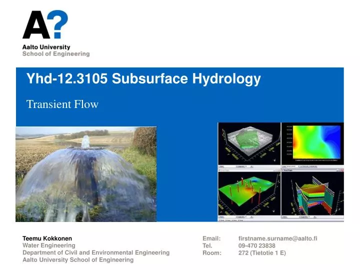
Yhd-12.3105 Subsurface Hydrology. Transient Flow. Teemu Kokkonen. Email : firstname.surname@aalto.fi Tel. 09-470 23838 Room : 272 (Tietotie 1 E). Water Engineering Department of Civil and Environmental Engineering Aalto University School of Engineering. Transient flow.

E N D
Yhd-12.3105 SubsurfaceHydrology TransientFlow Teemu Kokkonen Email: firstname.surname@aalto.fi Tel. 09-470 23838 Room: 272 (Tietotie 1 E) Water Engineering Department of Civil and Environmental Engineering Aalto UniversitySchool of Engineering
Transientflow t = 30 min t = 10 min t = 5 min • In a transient flow problem the hydraulic head values change with time t = 30 s t = 10 s Pumping well Q t = 1 d t = 0 t = 1 h t = 2 h t = 12 h
Storage t = 30 min t = 10 min t = 5 min • To be able to describe transient flow we need the concept of storage to account for changes in the amount of water in a control volume t = 30 s t = 10 s Pumping well Q t = 1 d t = 0 t = 1 h t = 2 h t = 12 h
Step 1.Write the equation for the specificstorativity. GroundwaterFlowEquationTransient 3D Specificstorativity S0 volume of wateradded to storage, per unitvolume and per unitrise in hydraulichead Step 2.Usespecificstorativity to write the change in the volume of water per unitvolume and per unittime. Step 3.Complete the equationshownbelow (i.e. replace the questionmarkwithsomethingelse).
GroundwaterFlowEquationTransient 2D Storagecoefficient S volume of wateradded to storage, per unitarea and per unitrise in hydraulichead
GroundwaterFlowEquationTransient 2D How is the aboveequationsimplifiedwhen the aquifer is homogeneous and isotropic? CanTchangewithtime? When?
Storage • Unconfinedaquifer • The ratiobetween air and water in the pore spacechanges (i.e. air is displacewithwater, orviceversa) • Confinedaquifer • Mineralgrains of the soilmatrixarereorganisedaffecting the porosity of the aquifer • When the aquifercompressesmoremineralgrainsaresqueezed into a controlvolume and somewater is displaced out of it • Water is to someextentcompressible • An unconfinedaquiferhas a muchgreatercapacity to store and release waterthan a confinedaquifer
t-1 t t+1 NumericalSolution – TransientFlow time • Thisfarwehavenumericallyestimatedspatialderivativesappearing in the groundwaterequations – nowwealsoneed to dealwith a temporalderivative Forwarddifference Superscripts (t and t +1) refer to the serialnumber of the time-step
t-1 t t+1 NumericalSolution – TransientFlow time ”old” time-stepused in computingspatialderivatives x y Write the numericalapproximation for the aboveequation.
NumericalSolution – TransientFlow • Expressing the spatialderivativesusingonly ”old” hydraulicheadvaluesallows for leaving just oneunknown ”new” hydraulicheadvalue on the left-hand side of the equation and solvingitsvaluebased on known ”old” hydraulicheadvalues=> explicitsolution • Easy to constructbutcanlead to numericalproblems (instability) • Expressing the spatialderivativesusing ”new” hydraulicheadvaluesleads to an implicitsolution • Numericallymorestablethen the explicitsolutionbutmoretedious to solve (requiresitaration) • Often a weightedaverage of derivativeswith ”old” and ”new” headvalues is used
ForwardProblem vs. InverseProblem • In a forwardproblem the hydraulicparameters (e.g. transimssivity) of an aquiferareknown and the problem is to simulate the hydraulicheadvalues • In an inverseproblemsomehydraulicheadvaluesareknown and the problem is to estimatevalues of hydraulicparameters • Scale problem: hydraulic properties estimated from small-sized soil samples may represent poorly hydraulic properties at a larger scale
Well-PosedProblem vs. Ill-posedProblem • In a well-posedproblem the followingcriteriaaremet • Existence: a solutionexists • Uniqueness: there is onlyonesolution • Stability: a change in the solution is smallif a change in hydraulicparameters is small • As opposed to the well-posedproblem, in an ill-posedproblem the abovecriteriaarenotmet
InverseProblem • Existence of solution • A mathematicalmodel is alwaysonly an approximation of the naturalsystemitdescribes • Measuredhydraulicheadvaluesarenoterror-free • For thesereasons the inverseproblemdoesnothave an exactsolution • The lack of exactsolution is notreally a problem • Uniqueness of the solution • k * 0 = 0 => k = ? • 2a + 3b = 10 => a = ? b = ? • Differenthydrogeologicalconditionscanresult in similarhydraulicheadvalues => the inversegroundwaterproblemoftendoesnothave a uniquesolution • Stability • The inversegroundwaterproblemoftensuffersfrominstabilityproblems
Pumpingtests • Pumpingtestsareused ”stimulate” the aquifer to getdrawdown data wherethere is something happening in the aquifer and whichgives a betterbasis to estimatehydrogeologicalparameters (exciting the system) • Typically in a pumpingtest the pumpingwell is pumped at a constantrate and the drawdownvaluesarerecorded as a function of time in observationwells at differentdistances • The pumpingtestresultscanbeinterpretedeitherusinginversemodelling, orwhensomesimplifiedassumptionsarevalidusinganalyticalsolutions
TheisMethod • Theis (1935) constructed a method to estimatetransmissivity and storagecoefficient of an aquiferfrompumpingtestresults • Assumptions • Homogeneous, isotropic, confined aquifer • The well is fullypenetrating • A constantpumpingrate • Infinitearealextent • Horizontalflow • Impermeable and horizontaltop and bottom boundaries of aquifer
TheisMethod H0 - H = drawdown, Q = pumping rate, T = transmissivity and W(u) on the well function, where r = distance from pumping well, S = storage coefficient and t is time from start of pumping Now The graphwheredrawdown is plotted as a function of timehas the sameshape as the graphwhere W(u) is plottedagainst 1/u.
TheisMethod • Plot the well function W(u) against 1/u:ta in a log-log scale (type curve) • Plot the measured drawdown values H0-Hagainst time t in a log-log scale (field curve) • Overlay the type curve and field curve – keeping the axes parallel – in such a way that the curves overlap as closely as possible • Select a match point (does not need to be on the curves) and read values W(u), 1/u, H0-Hand t • Use the equations shown a couple of slides back to calculate values for T and S