Download

1 / 57
890 likes | 1.7k Vues
CHI SQUARE TEST. DR HAR ASHISH JINDAL JR. Contents. Definitions Milestone in Statistics Chi square test Chi Square test Goodness of Fit Chi square test for homogeneity of Proportion Chi Square Independent test Limitation of Chi square Fischer Exact test Continuity correction

E N D
CHI SQUARE TEST DR HAR ASHISH JINDAL JR
Contents • Definitions • Milestone in Statistics • Chi square test • Chi Square test Goodness of Fit • Chi square test for homogeneity of Proportion • Chi Square Independent test • Limitation of Chi square • Fischer Exact test • Continuity correction • Overuse of chi square
Definitions • Statistics defined as the science, which deals with collection, presentation, analysis and interpretation of data. • Biostatistics defined as application of statistical method to medical, biological and public health related problems.
Statistics Inferential Descriptive Chi Square Test • Making inference • Hypothesis testing • Determining relationships • Making predictions • Collecting • Organizing • Summarizing • Presenting Data
Introduction • Data : A collection of facts from which conclusions can be made. • An observations made on the subjects one after the other is called raw data • It becomes useful - when they are arranged and organized in a manner that we can extract information from the data and communicate it to others.
Definitions • Avariable is any characteristics, number, or quantity that can be measured or counted. • Independent variable: doesn’t changed by the other variables. E.g age • Dependent variable: depends on other factors e.g test score on time studied • Parameter: is any numerical quantity that characterizes a given population or some aspect of it. E.g mean
Data Types • Interval data ` • Ratio data
Qualitative Data • Qualitative variables • Example: gender (male, female) • Frequency in category • Nominal or ordinal scale • Examples • Do you have a disease? - nominal • What is the Socio economic status ? – ordinal
MILESTONE IN STATISTICS • "Karl Pearson's famous chi-square paper appeared in the spring of 1900, an auspicious beginning to a wonderful century for the field of statistics." (published in the Philosophical magazine )
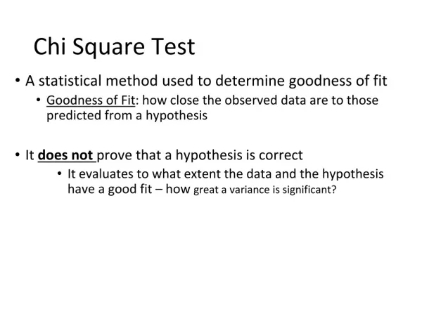
Chi Square Test • Simplest & most widely used non-parametric test in statistical work.
Logic of the chi-square • The total number of observations in each column and the total number of observations in each row are considered to be given or fixed. • If we assume that columns and rows are independent, we can calculate - expected frequencies.
Logic of Chi square • Compares the observed frequency in each cell with the expected frequency. If no relationship exists between the column and row variable If a relationship (or dependency) does occur the observed frequencies will be very close to the expected frequencies The observed frequencies will vary from the expected frequencies they will differ only by small amounts The value of the chi-square statistic will be large. the value of the chi-square statistic will be small
Steps for Chi square test Define Null and alternative hypothesis State alpha Calculate degree of freedom State decision rule Calculate test statistics State and Interpret results
Hypothesis Testing • Testsa claim about a parameter using evidence (data in a sample) gives causal relationships Steps • Formulate Hypothesis about the population • Random sample • Summarizing the information (descriptive statistic) • Does the information given by the sample support the hypothesis? Are we making any error? (inferential stat.) • Decision rule: Convert the research question to null and alternative hypothesis
Null Hypothesis • H0 = No difference between observed and expected observations • H1 = difference is present between observed and expected observations
What is statistical significance? • A statistical concept indicating that the result is very unlikely due to chance and, therefore, likely represents a true relationship between the variables. • Statistical significance is usually indicated by the alpha value (or probability value), which should be smaller than a chosen significance level.
State alpha value • Alpha is error(type I) that is • Rejecting a true null hypothesis • For majority of the studies alpha is 0.05 • Meaning: the investigator has set 5% as the maximum chance of incorrectly rejecting the null hypothesis
Degree of freedom • Calculation • For Goodness of Fit = Number of levels (outcome)-1 • For independent variables / Homogeneity of proportion : (No. of columns – 1) (No. of rows – 1) It is positive whole number that indicates the lack of restrictions in calculations. The degree of freedom is the number of values in a calculation that can vary.
The Chi-Square Distribution • No negative values • Mean is equal to the degrees of freedom • The standard deviation increases as degrees of freedom increase, so the chi-square curve spreads out more as the degrees of freedom increase. • As the degrees of freedom become very large, the shape becomes more like the normal distribution.
The Chi-Square Distribution • The chi-square distribution is different for each value of the degrees of freedom, different critical values correspond to degrees of freedom. • we find the critical value that separates the area defined by α from that defined by 1 – α.
If ni = E(ni), 2 = 0 Do not reject H0 Reject H0 = 0.05 c 2 5.991 0 2 Table (Portion) Significance level DF 0.995 … 0.95 … 0.05 1 ... … 0.004 … 3.841 2 0.010 … 0.103 … 5.991 Finding Critical Value Q. What is the critical 2value if df = 2, and =0.05? df =2
State decision rule If the value obtained is greater than the critical value of chi square , the null hypothesis will be rejected
Calculate test statistics Expected Value • Calculated using the formula- χ2 = ∑ ( O – E )2 E O = observed frequencies E = expected frequencies Chi square for independent variables Chi square for goodness of fit Homogeneity of proportion • Expected Value = Row total * Column total / Table total • a theory • Previous study • Comparison groups • Previous study • standard Question >>> How to find the Expected value
State and interpret results • See whether the value of chi square is more than or less than the critical value If the value of chi square is less than the critical value we accept the null hypothesis If the value of chi square is more than the critical value the null hypothesis can be rejected
Chi square test • Goodness of fit • For homogeneity of Proportions • For 2 independent groups • Cohort Study • Case control study • Matched case control Study • For > 2 independent groups
Goodness of fit Expected frequency can be based on • theory • previous experience • comparison groups Q How "close" are the observed values to those which would be expected in a study OR Q.whether a variable has a frequency distribution compariable to the one expected. Chi-square goodness of fit test
Goodness of fit • A goodness-of-fit test is an inferential procedure used to determine whether a frequency distribution follows a claimed distribution. • It is a test of the agreement or conformity between the observed frequencies (Oi) and the expected frequencies (Ei) for several classes or categories (i)
Example :Is Sudden Infant Death Syndrome seasonal?? Null Hypothesis: The proportion of deaths due to SIDS in winter , summer , autumn , spring is equal = ¼ = 25% Alternative :Not all probabilities stated a in null hypothesis is correct For α =0.05 for df =3 critical value X2 = 7.81 X2 = (78-80.5)2/80.5 + (71- 80.5)2/80.5 + (87.5 – 80.5)2/80.5 + (86 – 80.5)2/80.5 = 2.09 Degree of freedom = k-1 = 4-1 =3 Conclusion: As calculated X2 value is less than Critical value we can accept the null hypothesis and state that deaths due to SIDS across seasons are not statistically different from what's expected by chance (i.e. all seasons being equal)
Chi square test • Goodness of fit • For homogeneity of Proportions • For 2 independent groups • Cohort Study • Case control study • Matched case control Study • For > 2 independent groups
Homogeneity of proportions • In a chi-square test for homogeneity of proportions, we test the claim that different populations have the same proportion of individuals with some characteristic. EXAMPLE: Is there evidence to indicate that the perception of effects of vaccination is the same in 2013 as was in 2000? Q what is the effect of vaccination on health ? Answers :- Good , No , Bad Null hypothesis: Ho = No difference between the two population H1 = There is difference between the two population
State alpha = 0.05 find df = (3-1)(2-1)= 2 =5.99 Chi square distribution X2= 5.991
2000 2013 Good- 726 No-222 Bad -50 Good -656 No- 283 Bad- 50
Homogeneity of proportions • χ2 value = ∑ (O-E)2/E Calculated χ2= 10.871 Results: as 10.871> 5.991 we reject the null hypothesis at 0.05 significance . >There is a statistically significant difference in the level of feeling towards vaccination between 2000 and 2013
Chi square test • Goodness of fit • For homogeneity of Proportions • For 2 independent groups • Cohort Study • case control study • Matched case control Study • For > 2 independent groups
Chi square Independence test • It is used to find out whether there is an associationbetween a row variable and column variable in a contingency table constructed from sample data.
Assumption • The variables should be independent. • All expected frequencies are greater than or equal to 1 (i.e., E>1.) • No more than 20% of the expected frequencies are less than 5 Calculated as χ2 value = ∑ (O-E)2/E
a+b tt Joint probability = Marginal probability = a+b tt a+c tt Location DiseaseDiseaseExposure presentneg. Total Present a b a+ b Negativec dc + d Total a+cb+d tt a+b tt a+ctt Expected count = sample size Expected Count a+c tt Marginal probability = (tt)
Short cut of Chi Square Observed values Expected values
=> (37- 22.5)2/22.5 +(13 – 27.5)2/27.5 +(17-31.5)2 /31.5+ (53-38.5)2/38.5 = 29.1 • 120[(37)(53)-(13)(17)]2 • / 54(66)(50)(70) • = 29.1
Application in various studies • Cohort study • Case control study • Matched case control study
Cohort Study • Assumptions: • The two samples are independent • Let a+b = number of people exposed to the risk factor • Let c+d = number of people not exposed to the risk factor Assess whether there is association between exposure and disease by calculating the relative risk (RR)
Example: To test the association in a cohort study among smoking and Lung CA We can define the relative risk of disease: p1= (Incidence of disease in exposure present) p2 = (Incidence of disease exposure absent) Relative risk RR= p1/p2 Hence for these studies RR= (a/a+ b)/(c/c + d) We can test the hypothesis that RR=1 by calculating the chi-square test statistic Null hypothesis :Ho= No association between Smoking and Lung CA (RR=1) H1 =Association present b/w smoking and Lung CA RR = (84/3000)/(87/5000)=1.21 Alpha value= 0.05 and df = 1 CONCLUSION:As the X2 > than 3.82 we reject the null hypothesis of RR=1 at 0.05 significance.
Case control study • Assumptions • The samples are independent • Cases = diseased individuals = a+c • Controls = non-diseased individuals = b+d Assess whether there is association between exposure and disease by calculating the odds ratio (OR)
Example: To test the association in a case control study between CHD and smoking Null hypothesis Ho: No association between CHD and smoking(OR=1) H1= Association exists between CHD and Smoking(OR>1 or<1) • Odd’s Ratio = odd’s of exposure amongst diseased group/ odd’s of exposure amongst non diseased • odd’s of exposure amongst diseased = (a/a+c)/(c/a+c) = a/c • Odd’s of exposure amongst non diseased = (b/b+d)/(d/b+d) = b/d • Odd’s Ratio = ad/ bc • We can test whether OR=1 by calculating the chi-square Odd’s Ratio=112*224/88*176 = 1.62 Alpha value= 0.05 and df = 1 Conclusion: we reject the null hypothesis that odd’s ratio = 1 at 0.05 significance as X2 > 3.84
Matched case control study • Case-control pairs are matched on characteristics such as age, race, sex • Assumptions • Samples are not independent • The discordant pairs are case-control pairs with different exposure histories • The matched odds ratio is estimated by bb/cc • Pairs in which cases exposed but controls not = bb • Pairs in which controls exposed but cases not = cc Assess whether there is association between exposure and disease by calculating the matched odds ratio (OR)
To test association of smoking exposure and CHD in a matched case control study Null hypothesis : No association of smoking exposure and CHD (OR=1) Alternative Hypothesis: Association exists between smoking exposure and CHD(OR>1 or< 1) CHD absent • Test whether OR = 1 by calculating McNemar’s statistic CHD present Alpha value= 0.05 and df = 1 OR=40/10 = 4 X2= [(40-10)-1]2/(40+10) = 841/50 = 16.81 Conclusion: We reject the Null Hypothesis that OR =1 as calculated X 2>3.84
Chi square for > 2 independent variables • The chi-square test is used regardless of whether the research question in terms of proportions or frequencies • Contingency tables can have any number of rows and columns. • The sample size needs to increase as the number of categories increases to keep the expected values of an acceptable size.