Download
1 / 137
1.37k likes | 1.48k Vues
Galaxies II – Dr Martin Hendry. 10 lectures to A3/A4, beginning January 2008. Galaxies II – Dr Martin Hendry. 10 lectures to A3/A4, beginning January 2006 Course Topics. 1. Galaxy Kinematics. Spectroscopy and the LOSVD Measuring mean velocities and velocity dispersions

E N D
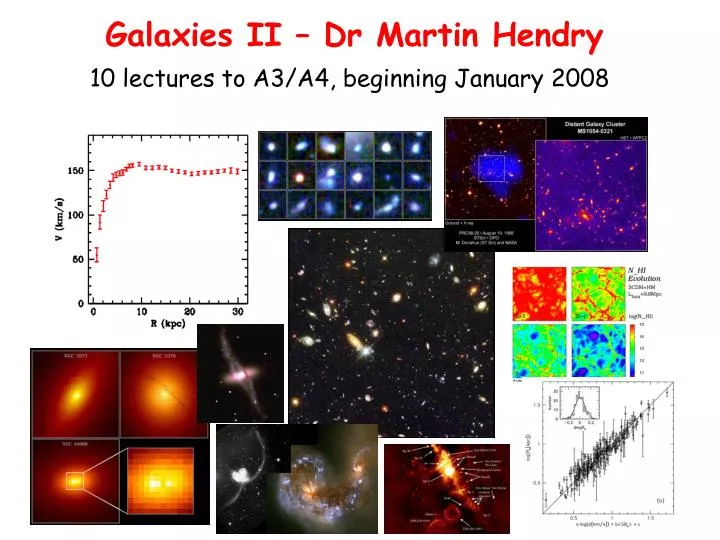
Galaxies II – Dr Martin Hendry 10 lectures to A3/A4, beginning January 2008
Galaxies II – Dr Martin Hendry 10 lectures to A3/A4, beginning January 2006 Course Topics 1. Galaxy Kinematics • Spectroscopy and the LOSVD • Measuring mean velocities and velocity dispersions • Rotation curves of disk systems • Evidence for dark matter halos • The Tully-Fisher and Fundamental Plane relations
2. Abnormal and Active Galaxies • Starburst galaxies • Galaxies with AGN • The unified model of AGN • Radio lobes and jets • Evidence for supermassive black holes Galaxies II – Dr Martin Hendry 10 lectures to A3/A4, beginning January 2006 Course Topics 1. Galaxy Kinematics • Spectroscopy and the LOSVD • Measuring mean velocities and velocity dispersions • Rotation curves of disk systems • Evidence for dark matter halos • The Tully-Fisher and Fundamental Plane relations
Galaxies II – Dr Martin Hendry 10 lectures to A3/A4, beginning January 2006 Course Topics 3. Galaxy Formation and Evolution • Galaxy mergers and interactions • Polar rings, dust lanes and tidal tails • Star formation in ellipticals and spirals • Chemical evolution models
Galaxies II – Dr Martin Hendry 10 lectures to A3/A4, beginning January 2006 Course Topics 3. Galaxy Formation and Evolution • Galaxy mergers and interactions • Polar rings, dust lanes and tidal tails • Star formation in ellipticals and spirals • Chemical evolution models 4. Galaxies and Cosmology • Hierarchical clustering theories • Galaxy clusters as cosmological probes • Proto-galaxies and the Lyman-alpha forest • Re-ionisation of the early Universe
Some Relevant Textbooks (Not required for purchase, but useful for consultation) • An Introduction to Modern Astrophysics, • B.W. Carroll & D.A. Ostlie (Addison-Wesley) • Galactic Astronomy, • J. Binney & M. Merrifield (Princeton UP) • Galactic Dynamics, • J. Binney & S. Tremaine (Princeton UP) • Galaxies and the Universe, • L. Sparke & J.S. Gallagher (Cambridge UP)
1. Kinematics of Galaxies The key to probing large-scale motions within galaxies is spectroscopy Radiation emitted from gas (e.g. stars, nebulae) moving radially is Doppler shifted
1. Kinematics of Galaxies The key to probing large-scale motions within galaxies is spectroscopy Radiation emitted from gas (e.g. stars, nebulae) moving radially is Doppler shifted Radial velocity (can be +ve or –ve) Change in wavelength (can be +ve or –ve) (1.1) Wavelength of light as measured in the laboratory Speed of light (Formula OK if v << c)
Radial velocity (can be +ve or –ve) Change in wavelength (can be +ve or –ve) Wavelength of light as measured in the laboratory Speed of light 1. Kinematics of Galaxies The key to probing large-scale motions within galaxies is spectroscopy Radiation emitted from gas (e.g. stars, nebulae) moving radially is Doppler shifted Analysis of individual spectral lines can allow measurement of line of sight velocity (1.1) Fine for individual stars (e.g. spectroscopic binaries – recall A1Y stellar astrophysics) (Formula OK if v << c)
Spectroscopic Binaries Orbits, from above B A A B B A B A To Earth Spectral lines B A A+B A B A+B
When we collect light from some small projected area of a galaxy, its spectrum is the sum of spectra from stars and gas along that line of sight – all with different line of sight velocities. This ‘smears out’ individual spectral lines
When we collect light from some small projected area of a galaxy, its spectrum is the sum of spectra from stars and gas along that line of sight – all with different line of sight velocities. This ‘smears out’ individual spectral lines (Not really a problem for determining cosmological redshifts for distant galaxies, since broadening of spectral lines across galaxy is a small effect compared with the radial velocity of entire galaxy. See e.g. Lyman Ha line: SDSS)
When we collect light from some small projected area of a galaxy, its spectrum is the sum of spectra from stars and gas along that line of sight – all with different line of sight velocities. This ‘smears out’ individual spectral lines We define the Line of Sight Velocity Distribution (LOSVD) via: Fraction of stars contributing to spectrum with radial velocities between and (1.2)
It is useful to define the observed spectrum not in terms of wavelength or frequency, but spectral velocity, , via (1.3)
It is useful to define the observed spectrum not in terms of wavelength or frequency, but spectral velocity, , via Hence, a Doppler shift of corresponds to (1.3) (1.4)
It is useful to define the observed spectrum not in terms of wavelength or frequency, but spectral velocity, , via Hence, a Doppler shift of corresponds to Light observed at spectral velocity was emitted at spectral velocity (1.3) (1.4)
Suppose that all stars have intrinsically identical spectra, measures the (relative) intensity of radiation at spectral velocity Intensity received from a star with line of sight velocity is Relative intensity (arbitrary units) Wavelength (Angstroms)
Suppose that all stars have intrinsically identical spectra, measures the (relative) intensity of radiation at spectral velocity Intensity received from a star with line of sight velocity is Relative intensity (arbitrary units) Observed composite spectrum: Wavelength (Angstroms) (1.5)
Suppose that all stars have intrinsically identical spectra, measures the (relative) intensity of radiation at spectral velocity Intensity received from a star with line of sight velocity is Observed composite spectrum: (1.5)
Suppose that all stars have intrinsically identical spectra, measures the (relative) intensity of radiation at spectral velocity Intensity received from a star with line of sight velocity is Observed composite spectrum: Galaxy spectrum is smoothed version of stellar spectrum – ‘smeared out’ by LOSVD (1.5)
Spectral Synthesis (See Section 3) Of course, stars don’t all have identical spectra, replaced by (local) average spectrum which depends on : • age • metallicity • galaxy environment
Spectral Synthesis (See Section 3) Of course, stars don’t all have identical spectra, replaced by (local) average spectrum which depends on : • age • metallicity • galaxy environment (1.6)
Spectral Synthesis (See Section 3) Of course, stars don’t all have identical spectra, replaced by (local) average spectrum which depends on : • age • metallicity • galaxy environment We consider here only the simpler case where is the same throughout the galaxy
Generally the slowly varying continuum component of the spectrum is removed first – i.e. we write: Emission: Absorption: (1.7)
Generally the slowly varying continuum component of the spectrum is removed first – i.e. we write: so that Emission: Absorption: (1.7) (1.8)
Generally the slowly varying continuum component of the spectrum is removed first – i.e. we write: so that Emission: Absorption: (1.7) (1.8) Relative intensity (arbitrary units) Wavelength (Angstroms)
Equation (1.8) is an example of an integral equation, where the function we can observe (the galaxy spectrum) is related to the integral of the function we wish to determine (the LOSVD). Observed galaxy spectrum ‘Template’ stellar spectra LOSVD
Equation (1.8) is an example of an integral equation, where the function we can observe (the galaxy spectrum) is related to the integral of the function we wish to determine (the LOSVD). It is a particular type of integral equation: a convolution Observed galaxy spectrum ‘Template’ stellar spectra LOSVD (1.9) ‘Data’ function ‘Kernel’ function ‘Source’ function
We want to estimate the source function, , given the observed galaxy spectrum, , and using a kernel function, , computed from e.g. a stellar spectral synthesis model. How can we extract from inside the integral?…
We want to estimate the source function, , given the observed galaxy spectrum, , and using a kernel function, , computed from e.g. a stellar spectral synthesis model. How can we extract from inside the integral?… Fourier Convolution Theorem Consider a convolution equation of the form The Fourier transforms of the functions , and satisfy the relation Here (1.10) For proof, see Examples 1
In the context of our problem: And Hence, we can in principle invert the integral equation and reconstruct the LOSVD, (1.11) (1.12) Inverse Fourier transform
In the context of our problem: And Hence, we can in principle invert the integral equation and reconstruct the LOSVD, In practice, this method is vulnerable to noise on the observed galaxy spectrum, , and uncertainties in the kernel . Need to filter out high frequency (k) noise (1.11) (1.12) Inverse Fourier transform
Filter, denoting range of wavenumbers which give reliable inversion Ratio of two small quantities: very noisy
If we cannot easily reconstruct the complete LOSVD , we can at least constrain some of the simplest properties of this function (1.13) Mean value (1.14) Variance (1.15) Velocity dispersion
The Cross-Correlation Function Method This is a common method for estimating and . Pioneered by e.g. Tonry & Davis (1979) We define: (We use continuum-subtracted galaxy and template spectra) (1.16)
The Cross-Correlation Function Method For a random value of the product fluctuates between +ve and –ve values is small +ve -ve +ve -ve
The Cross-Correlation Function Method For a random value of the product fluctuates between +ve and –ve values is small +ve -ve +ve -ve
The Cross-Correlation Function Method For a random value of the product fluctuates between +ve and –ve values is small +ve -ve +ve -ve
The Cross-Correlation Function Method For a random value of the product fluctuates between +ve and –ve values is small +ve -ve +ve -ve
The Cross-Correlation Function Method When emission and absorption features line up, and the product is large everywhere is large and positive +ve -ve +ve -ve
The Cross-Correlation Function Method We estimate by finding the maximum of the cross-correlation function.
The Cross-Correlation Function Method We estimate by finding the maximum of the cross-correlation function. Width of CCF peak allows estimation of Advantages: Fast, objective, automatic
What do we learn from the LOSVD?… In the Milky Way, analysis of HI 21cm radio emission, has revealed the spiral structure of the Galaxy (See A1Y Cosmology and A2 Theoretical Astrophysics)
What do we learn from the LOSVD?… In the Milky Way, analysis of HI 21cm radio emission, has revealed the spiral structure of the Galaxy (See A1Y Cosmology and A2 Theoretical Astrophysics)
What do we learn from the LOSVD?… In the Milky Way, analysis of HI 21cm radio emission, has revealed the spiral structure of the Galaxy Can also probe spiral structure from spectra of HII regions HII region = ISM region surrounding hot young stars (O and B) in which hydrogen is ionised. These trace out spiral arms, where young stars are being born Examples: Orion Nebula, Great Nebula in Carina
What do we learn from the LOSVD?… In the Milky Way, analysis of HI 21cm radio emission, has revealed the spiral structure of the Galaxy Can also probe spiral structure from spectra of HII regions Other MW tracers include: CO in molecular clouds H2O masers Cepheids, RR Lyraes Globular Clusters
What do we learn from the LOSVD?… We can construct a rotation curve : a graph of rotation speed versus distance from the centre of the galaxy. Milky Way Rotation Curve
Inside 1 kpc ‘rigid-body’ rotation This is consistent with a spherical matter distribution, of constant matter density Consider a mass, , at distance from the centre of the Galaxy. Equating circular acceleration and gravitational force: (1.17) Mass interior to radius r