Download
1 / 55
550 likes | 652 Vues
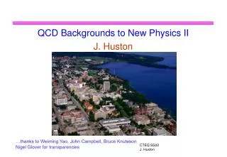
QCD Backgrounds to New Physics I J. Huston. …thanks to Weiming Yao, John Campbell, Bruce Knuteson Nigel Glover for transparencies. Home again. don’t worry about the extra o. Houston Renfrewshire A large village located 6 miles (9.6 km) north-west of Paisley, the name derives

E N D
QCD Backgrounds to New Physics I J. Huston …thanks to Weiming Yao, John Campbell, Bruce Knuteson Nigel Glover for transparencies
Home again don’t worry about the extra o Houston Renfrewshire A large village located 6 miles (9.6 km) north-west of Paisley, the name derives from 'Hew's town', a 13th century village around the castle of Hugo de Kilpeter. In 1781 the castle was partly demolished and a New Town of 35 houses was erected. The Crosslee Mill (1793, demolished 1986) was used for cotton spinning but in 1916-17 a new factory was constructed for 'spinning cordite fuses'. The Mercat Cross has a sundial from the early 18th century and a shaft which may be 14th century; Houston House (17th century) and Barochan House (17th century and 1896) are other notable buildings.
Run 2 Monte Carlo Workshop • Transparencies, video links to individual talks and links to programs can all be found at http://www-theory.fnal.gov/runiimc/ • I’ll be referring to some of these programs in the course of my talk
Les Houches • Two workshops on “Physics at TeV Colliders” have been held so far, in 1999 and 2001 (May 21-June 1) • Working groups on QCD/SM, Higgs, Beyond Standard Model • See web page: http://wwwlapp.in2p3.fr/conferences/LesHouches/Houches2001/ especially for links to writeups from 1999 • QCD writeup (hep-ph/0005114) is an excellent pedagogical review for many of the issues discussed here and at this SS
Other useful references (for pdf uncertainties) • LHC Guide to Parton Distributions and Cross Sections, J. Huston; http://www.pa.msu.edu/~huston/lhc/lhc_pdfnote.ps • The QCD and Standard Model Working Group: Summary Report from Les Houches; hep-ph/0005114 • Parton Distributions Working Group, Tevatron Run 2 Workshop; hep-ph/0006300 • A QCD Analysis of HERA and fixed target structure function data, M. Botje; hep-ph/9912439 • Global fit to the charged leptons DIS data…, S. Alekhin; hep-ph/0011002 • Walter Giele’s presentation to the QCD group on Jan. 12; http://www-cdf.fnal.gov/internal/physics/qcd/qcd99_internal_meetings.html • Uncertainties of Predictions from Parton Distributions I: the Lagrange Multiplier Method, D. Stump, J. Huston et al.;hep-ph/0101051 • Uncertainties of Predictions from Parton Distributions II: the Hessian Method, J. Pumplin, J. Huston et al.; hep-ph/0101032
Other references… …to the ability to calculate QCD backgrounds …to the need to do so
One person was more offended by the book than Carlo Rubbia • “Stirling was a dapper Englishman, in his mid-thirties…” p. 228
UA1 monojets (1983-1984) Possible signature of new physics (SUSY, etc) A number of backgrounds were identified, but each was noted as being too small to account for the observed signal pp->Z + jets |_ nn pp->W + jets |_ t + n |_ hadrons + n pp->W + jets |_ l + n pp->W + jets |_ t + n |_ l + n …but the sum was not “The sum of many small things is a big thing.” G. Altarelli Can calculate from first principles or calibrate to observed cross sections for Z->e+e- and W->en Ellis, Kleiss, Stirling PL 167B, 1986. Monojets in UA1 jet
Signatures of New Physics • W’s, jets, g’s, b quarks, ET • …pretty much the same as signatures for SM physics • How do we find new physics? By showing that it’s not old physics. • can be modifications to the rate of production • …or modification to the kinematics, e.g.angular distributions • Crucial to understand the QCD dynamics of both backgrounds to any new physics and to the new physics itself • Some backgrounds can be measured in situ • …but may still want to predict in advance, e.g. QCD backgrounds to H->gg • For some backgrounds, need to rely on theoretical calculations, e.g. ttbb backgrounds to ttH
Theoretical Predictions for New (Old) Physics There are a variety of programs available for comparison of data to theory and/or predictions. • Tree level • Leading log Monte Carlo • NnLO • Resummed Important to know strengths/weaknesses of each. In general, agree quite well…but before you appeal to new physics, check the ME. (for example using Comphep) Can have ME corrections to MC or MC corrections to ME. (in CDF->HERPRT) Perhaps biggest effort…include NLO ME corrections in Monte Carlo programs… correct normalizations. Correct shapes. NnLO needed for precision physics. Resummed description describes soft gluon effects (better than MC’s)…has correct normalization (but need HO to get it); resummed predictions include non-perturbative effects correctly…may have to be put in by hand in MC’s b space (ResBos) threshold kT W,Z, Higgs dijet, direct g qt space Where possible, normalize to existing data. …in addition, worry about pdf, fragmentation uncertainties
W + Jet(s) at the Tevatron • Good testing ground for parton showers, matrix elements, NLO • Background for new physics • or old physics (top production) • Reasonable agreement for the leading order comparisons using VECBOS (but large scale dependence) • Good agreement with NLO (and smaller • scale dependence) for W + >= 1 jet
W + jets • For W + >=n jet production, typically use Herwig (Herprt) for additional gluon radiation and for hadronization • Can also start off with n-1 jets and generate additional jets using Herwig
More Comparisons (VECBOS and HERWIG) • Start with W + (n-1) jets from VECBOS • Start with W + n jets from VECBOS
More Comparisons • Start with W + n jets from VECBOS • Start with W + (n-1) jets from VECBOS
Consider W + jet(s) sample Compare data (Run 0 CDF) to VECBOS+HERPRT (Herwig radiation+hadronization interface to VECBOS) normalized to W+X jets Starting with W + 1 jet rate in data, Herwig predicts 1 W+ >4 jet events; in data observe 10 …factor of ~2 every jet very dependent on kinematic situation, though jet ET cuts center-of-mass energy etc #events >1 jet >2 jets >3 jets >4 jet pT>10 GeV/c Data 920 213 42 10 VECBOS + HERPRT (Q=<pT>) W + 1jet 920 178 21 1 W + 2jet ----- 213 43 6 W + 3jet ----- ----- 42 10 VECBOS+HERPRT(Q=mW) W + 1jet 920 176 24 2 W + 2jet ---- 213 46 6 W + 3 jet ---- ----- 42 7 When good Monte Carlos go bad
Why? • Some reasons given by the experts (Mangano, Yuan,Ilyin…) • Herwig (any Monte Carlo) only has collinear part of matrix element for gluon emission; underestimate for the wide angle emission that leads to widely separated jets • phase space: Herwig has ordering in virtualities for gluon emission while this is not present in exact matrix element calculations; more phase space for gluon emission in exact matrix element calculations • in case of exact matrix element, there are interferences among all of the different diagrams; these interferences become large when emissions take place at large angles (don’t know a priori whether interference is positive or negative) • unitarity of Herwig evolution: multijet events in Herwig will always be a fraction of the 2 jet rate, since multijet events all start from the 2-jet hard process • all “K-factors” from higher order are missed.
Leading order matrix element calculations describe multi-body configurations better than parton showers Many programs exist for calculation of multi-body final states at tree-level references at beginning of talk; see Run 2 MC workshop CompHep includes SM Lagrangian and several other models, including MSSM deals with matrix elements squared calculates leading order 2->4-6 in the final state taking into account all of QCD and EW diagrams color flow information; interface exits to Pythia great user interface Grace similar to CompHep Madgraph SM + MSSM deals with helicity amplitudes “unlimited” external particles (12?) color flow information not much user interfacing yet Alpha + O’Mega does not use Feynman diagrams gg->10 g (5,348,843,500 diagrams) Tree Level Calculations
To obtain full predictability for a theoretical calculation, would like to interface to a Monte Carlo program (Herwig, Pythia, Isajet) parton showering (additional jets) hadronization detector simulation Some interfaces already exist VECBOS->Herwig (HERPRT) CompHep->Pythia A general interface accord was reached at the 2001 Les Houches workshop All of the matrix element programs mentioned will output 4-vector and color flow information in such a way as to be universally readable by all Monte Carlo programs CompHep, Grace, Madgraph, Alpha, etc, etc ->Herwig, Pythia, Isajet Monte Carlo Interfaces
Parton Showering Note the large difference between PYTHIA versions 5.7 and 6.1. Which one is correct? • Determination of the Higgs signal requires an understanding of the Higgs pT distribution at both LHC and Tevatron • for example, for gg->HX->ggX, the shape of the signal pT distribution is harder than that of the gg background; this can be used to advantage • To reliably predict the Higgs pT distribution, especially for low to medium pT region, have to include effects of soft gluon radiation • can either use parton showering a la Herwig, Pythia, ISAJET or kT resummation a la ResBos • parton showering resums primarily the (universal) leading logs while an analytic kT resummation can resum all logs with Q2/pT2 in their arguments; but expect predictions to be similar and Monte Carlos offer a more useful format • Where possible it’s best to compare pT predictions to a similar data set to insure correctness of formalism; if data is not available, compare MC’s to a resummed calculation or at least to another Monte Carlo • all parton showers are not equal
Change in PYTHIA S. Mrenna 80 GeV Higgs generated at the Tevatron with Pythia • Older version of PYTHIA has more events at moderate pT • Two changes from 5.7 to 6.1 • A cut has been placed on the combination of z and Q2 values in a branching: u=Q2-s(1-z)<0 where s refers to the subsystem of hard scattering plus shower partons • corner of emissions that do not respect this requirement occurs when Q2 value of space-like emitting parton is little changed and z value of branching is close to unity • necessary if matrix element corrections are to be made to process • net result is substantial reduction in amount of gluon radiation • In principle affects all processes; in practice only gg initial states • Parameter for minimum gluon energy emitted in space-like showers is modified by extra factor corresponding to 1/g factor for boost to hard subprocess frame • result is increase in gluon radiation • The above are choices, not bugs; which version is more correct? • ->Compare to ResBos
Comparison of PYTHIA and ResBos for Higgs Production at LHC • ResBos agrees much better with the more recent version of PYTHIA • Suppression of gluon radiation leading to a decrease in the average pT of the produced Higgs • Affects the ability of CMS to choose to the correct vertex to associate with the diphoton pair • Note that PYTHIA does not describe the high pT end well unless Qmax2 is set to s (14 TeV) • Again, ResBos has the correct matrix element matching at high pT; setting Qmax2=s allows enough additional gluon radiation to mimic the matrix element
Comparisons with Herwig at the LHC • HERWIG (v5.6) similar in shape in PYTHIA 6.1 (and perhaps even more similar in shape to ResBos) • Is there something similar to the u-hat cut that regulates the HERWIG behavior? • Herwig treatment of color coherence? (study in progress)
What would we like? Bruce Knuteson’s wishlist from the Run 2 Monte Carlo workshop …all at NLO
MCFM (Monte Carlo for Femtobarn Processes) J. Campbell and K.Ellis • Goal is to provide a unified description of processes involving heavy quarks, leptons and missing energy at NLO accuracy • There have so far been three main applications of this Monte Carlo, each associated with a different paper. • Calculation of the Wbb background to a WH signal at the Tevatron. R.K.Ellis, Sinisa Veseli, Phys. Rev. D60:011501 (1999), hep-ph/9810489. • Vector boson pair production at the Tevatron, including all spin correlations of the boson decay products. J.M.Campbell, R.K.Ellis, Phys. Rev. D60:113006 (1999), hep-ph/9905386. • Calculation of the Zbb and other backgrounds to a ZH signal at the Tevatron. J.M.Campbell, R.K.Ellis, FERMILAB-PUB-00-145-T, June 2000, hep-ph/0006304. The last of these references contains the most details of our method.
Recent example of data vs Monte Carlo • There is a discovery potential at the Tevatron during Run 2 for a relatively light Higgs (especially if Higgs mass is 115 GeV) • …but small signal to background ratio makes understanding of backgrounds very important • CDF and ATLAS recently went through similar exercises regarding this background • CDF using Run 1 data • ATLAS using Monte Carlo predictions
Sleuth strategy • Consider recent major discoveries in hep • W,Z bosons CERN 1983 • top quark Fermilab 1995 • tau neutrino Fermilab 2000 • Higgs Boson? CERN 2000 • In all cases, predictions were definite, aside from mass • Plethora of models that appear daily on hep-ph • Is it possible to perform a “generic” search? Transparencies from Bruce Knuteson talk at Moriond 2001
Sleuth Bruce Knuteson Step 1: Exclusive final states Steps: 1) We consider exclusive final states We assume the existence of standard object definitions These define e, μ, , , j, b, ET, W, and Z fi All events that contain the same numbers of each of these objects belong to the same final state W2j eETjj W3j eET3j ee eμET Z e W μμμ μμjj eμETj Z4j eee
Sleuth Bruce Knuteson Step 2: Variables 2) Define variables What is it we’re looking for? The physics responsible for EWSB What do we know about it? Its natural scale is a few hundred GeV What characteristics will such events have? Final state objects with large transverse momentum What variables do we want to look at? pT’s
Sleuth Bruce Knuteson Step 2: Variables If the final state contains Then consider the variable 1 or more lepton 1 or more /W/Z 1 or more jet missing ET (adjust slightly for idiosyncrasies of each experiment)
Sleuth Bruce Knuteson Step 3: Search for regions of excess 3) Search for regions of excess (more data events than expected from background) within that variable space For each final state . . . Input: 1 data file, estimated backgrounds • transform variables into the unit box • define regions about sets of data points • Voronoi diagrams • define the “interestingness” of an arbitrary region • the probability that the background within that region fluctuates up to or beyond the observed number of events • search the data to find the most interesting region, R • determine P, the fraction of hypothetical similar experiments (hse’s) in which you would see something more interesting than R • Take account of the fact that we have looked in many different places Output: R, P
Sleuth Bruce Knuteson Sensitivity If the data contain no new physics, Sleuth will find to be random in (0,1) If we find small, we have something interesting If the data contain new physics, Sleuth will hopefully find to be small If we find large, is there no new physics in our data? or have we just missed it? How sensitive is Sleuth to new physics? Impossible to answer, in general (Sensitive to what new physics?) But we can provide an answer for specific cases
Sleuth Bruce Knuteson Sensitivity tt provides a reasonable sensitivity check[cf. DØ PRL (1997, 125 pb-1)] in eμET 2j: find >2 in 25% of an ensemble of mock experiments [cf. dedicated search: 2.75 (3 events with 0.2 expected)] in W 4j: find >3 in 25% of an ensemble of mock experiments [cf. dedicated search: 2.6 (19 events with 8.7 expected) w/o b-tag] [cf. dedicated search: 3.6 (11 events with 2.5 expected) w/ b-tag] Would we have “discovered” top with Sleuth? No. But results are nonetheless encouraging. Lessons:b-tagging, combination of channels important for top other sensitivity checks (WW, leptoquarks) give similarly sensible results
Results DØ data Results agree well with expectation No evidence of new physics is observed
Conclusions • Sleuth is a quasi-model-independent search strategy for new high pT physics • Defines final states and variables • Systematically searches for and quantifies regions of excess • Sleuth allows an a posteriori analysis of interesting events • Sleuth appears sensitive to new physics • Sleuth finds no evidence of new physics in DØ data • Sleuth has the potential for being a very useful tool • Looking forward to Run II hep-ex/0006011 PRD hep-ex/0011067 PRD hep-ex/0011071 PRL
One of the most useful search modes for the discovery of the Higgs in the 100-150 GeV mass range at the LHC is in the two photon mode Higgs->gg has very large backgrounds from QCD sources Diphoton production po and popo production; jets fragmenting into very high z po’s With excellent diphoton mass resolution, can try to resolve Higgs “bump” Still important to understand level of background Fragmentation: Higgs->gg and Backgrounds
Diphoton Backgrounds in ATLAS • Again, for a H->gg search at the LHC, face irreducible backgrounds from QCD gg and reducible backgrounds from gpo and popo • in range from 70 to 170 GeV jet-jet cross section is estimated to be a factor of 2E6 times the gg cross section and g-jet a factor of 8E2 larger • Need rejection factors of 2E7 and 8E3 respectively • PYTHIA results seem to indicate that reducible backgrounds are comfortably less than reducible ones • …but how to normalize PYTHIA predictions for very high z fragmentation of jets; fragmentation not known well at high z and certainly not for gluon jets
Different models predict different high z fragmentation • Backgrounds to gg production in Higgs mass region arise from fragmentation of jets to high z po’s • Pythia and Herwig predict very different rates for high z • all fragmentation is not equal • Example of a background that can be measured in situ, but nice to be able to predict the environment beforehand • DIPHOX (see Run 2 MC workshop) program can calculate gg, gpo, and popo cross sections to NLO • comparisons underway to Tevatron data • gg->gg and qqbar->gg at NNLO may be available soon B. Webber, hep-ph/9912399
What’s unknown about PDF’s the gluon distribution strange and anti-strange quarks details in the {u,d} quark sector; up/down differences and ratios heavy quark distributions S of quark distributions (q + qbar) is well-determined over wide range of x and Q2 Quark distributions primarily determined from DIS and DY data sets which have large statistics and systematic errors in few percent range (±3% for 10-4<x<0.75) Individual quark flavors, though may have uncertainties larger than that on the sum; important, for example, for W asymmetry information on dbar and ubar comes at small x from HERA and at medium x from fixed target DY production on H2 and D2 targets Note dbar≠ubar strange quark sea determined from dimuon production in n DIS (CCFR) d/u at large x comes from FT DY production on H2 and D2 and lepton asymmetry in W production PDF Uncertainties
Example:Jets at the Tevatron • Both experiments compare to NLO QCD calculations • D0: JETRAD, modified Snowmass clustering(Rsep=1.3, mF=mR=ETmax/2 • CDF: EKS, Snowmass clustering (Rsep=1.3 (2.0 in some previous comparisons), mF=mR=ETjet/2 • In Run 1a, CDF observed an excess in the • jet cross section at high ET, outside the • range of the theoretical uncertainties shown
Non-exotic explanations Modify the gluon distribution at high x