Download
1 / 5
50 likes | 68 Vues
Computing and Statistical Data Analysis Stat 3: The Monte Carlo Method. London Postgraduate Lectures on Particle Physics; University of London MSci course PH4515. Glen Cowan Physics Department Royal Holloway, University of London g.cowan@rhul.ac.uk www.pp.rhul.ac.uk/~cowan.

E N D
Computing and Statistical Data Analysis Stat 3: The Monte Carlo Method London Postgraduate Lectures on Particle Physics; University of London MSci course PH4515 Glen Cowan Physics Department Royal Holloway, University of London g.cowan@rhul.ac.uk www.pp.rhul.ac.uk/~cowan Course web page: www.pp.rhul.ac.uk/~cowan/stat_course.html Computing and Statistical Data Analysis / Stat 3
The Monte Carlo method What it is: a numerical technique for calculating probabilities and related quantities using sequences of random numbers. The usual steps: (1) Generate sequence r1, r2, ..., rm uniform in [0, 1]. (2) Use this to produce another sequence x1, x2, ..., xn distributed according to some pdf f (x) in which we’re interested (x can be a vector). (3) Use the x values to estimate some property of f (x), e.g., fraction of x values with a < x < b gives → MC calculation = integration (at least formally) MC generated values = ‘simulated data’ →use for testing statistical procedures Computing and Statistical Data Analysis / Stat 3
Random number generators Goal: generate uniformly distributed values in [0, 1]. Toss coin for e.g. 32 bit number... (too tiring). →‘random number generator’ = computer algorithm to generate r1, r2, ..., rn. Example: multiplicative linear congruential generator (MLCG) ni+1 = (a ni) mod m , where ni = integer a = multiplier m = modulus n0 = seed (initial value) N.B. mod = modulus (remainder), e.g. 27 mod 5 = 2. This rule produces a sequence of numbers n0, n1, ... Computing and Statistical Data Analysis / Stat 3
Random number generators (2) The sequence is (unfortunately) periodic! Example (see Brandt Ch 4): a = 3, m = 7, n0 = 1 ← sequence repeats Choose a, m to obtain long period (maximum = m- 1); m usually close to the largest integer that can represented in the computer. Only use a subset of a single period of the sequence. Computing and Statistical Data Analysis / Stat 3
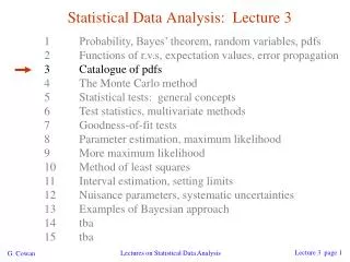
Random number generators (3) are in [0, 1] but are they ‘random’? Choose a, m so that the ri pass various tests of randomness: uniform distribution in [0, 1], all values independent (no correlations between pairs), e.g. L’Ecuyer, Commun. ACM 31 (1988) 742 suggests a = 40692 m = 2147483399 Far better generators available, e.g. TRandom3, based on Mersenne twister algorithm, period = 219937 - 1 (a “Mersenne prime”). See F. James, Comp. Phys. Comm. 60 (1990) 111; Brandt Ch. 4 Computing and Statistical Data Analysis / Stat 3