Download
1 / 50
500 likes | 1.03k Vues
Long-Term Space Weather and Terrestrial Climate. David H. Hathaway NASA/MSFC National Space Science and Technology Center Huntsville, AL 2004 December 17. Outline. Space Weather – What is it? Sunspots and the Sunspot Cycle Long Term Changes in Space Weather

E N D
Long-Term Space WeatherandTerrestrial Climate David H. Hathaway NASA/MSFC National Space Science and Technology Center Huntsville, AL 2004 December 17
Outline • Space Weather – What is it? • Sunspots and the Sunspot Cycle • Long Term Changes in Space Weather • Space Weather and Terrestrial Climate
Effects of Solar Activity: On Satellites Radiation (protons, electrons, alpha particles) from solar flares and coronal mass ejections can damage electronics on satellites. Heating of the Earth’s upper atmosphere increases satellite drag. • 1991 GOES • 1995 Deutsche Telekom • 1996 Telesat Canada • 1997 Telstar 401 • 2000/07/14 ASCA • 2003 Mars Odyssey • 4500 spacecraft anomalies over last 25 years
Effects of Solar Activity: On Power Grids Solar disturbances shake the Earth’s magnetic field. This sets up huge electrical currents in power lines and pipe lines. The solar storm of March 13th 1989 fried a $10M transformer in NJ. The same storm interrupted power to the province of Quebec for 6 days.
Effects of Solar Activity: On Radio Wave Propagation Variations in ionizing radiation (UV, EUV, X-rays) from the Sun alter the ionosphere – changing the Maximum Usable Frequency for high frequency radio communications and altering position information for GPS systems.
Sunspot Number International Sunspot Number – devised by Rudolf Wolf in the 1850s (1749-Present but incomplete before 1850) SSN = 10 G + N (G = # of Groups, N = # of spots) Group Sunspot Number – devised by Hoyt and Schatten in the 1990s (1610-Present more complete than Wolf’s sunspot number) GSSN = 12.08 G Sunspot numbers are also generated by NOAA in Boulder, CO and by the American Association of Variable Star Observers
The “11-year” Sunspot Cycle Cycle periods are normally distributed with a mean period of 131 months and a standard deviation of 14 months.
Sunspot Number and Solar Activity Sunspot number is well correlated with other measures of solar activity. The long record of sunspot numbers helps to characterize the solar cycle. Sunspot Area 10.7cm Radio Flux GOES X-Ray Flares Total Irradiance Geomagnetic aa index Climax Cosmic-Ray Flux
The Waldmeier Effect The sunspot cycles are asymmetric – the time to rise to maximum is less than the time to fall to minimum. Furthermore, large cycles take less time to reach maximum than do small cycles.
Amplitude-Period Effect The amplitude of a cycle is anti-correlated to the period of the previous cycle. Large cycles follow short cycles.
Amplitude-Minimum Effect The amplitude of a cycle is correlated with the size of the minimum that precedes the cycle.
Individual Cycle Characteristics Big cycles start early and grow fast. This directly produces the Waldmeier Effect. By doing so they cut short the previous cycle (Amplitude-Period Effect) and produce a higher minimum due to the overlap (Amplitude-Minimum Effect).
Understanding the Sunspot Cycle: Solar Magnetism
Hale’s Polarity Law The polarity of the preceding spots in the northern hemisphere is opposite to the polarity of the preceding spots in the southern hemisphere. The polarities reverse from one cycle to the next.
Sunspot Latitude Drift Sunspots appear in two bands on either side of the equator. These bands spread in latitude and then migrate toward the equator as the cycle progresses. Cycles often overlap around the time of minimum.
The Sun’s Magnetic Cycle This movie shows the equatorward drift of the active regions and Hale’s polarity law. It also reveals the differential rotation (faster at the equator, slower at high latitudes) and poleward meridional flow.
Polar Field Reversal at Cycle Maximum The polarity of the polar magnetic fields reverses at about the time of the solar activity maximum.
Active Region Tilt: Joy’s Law Active regions are tilted so that the following polarity spots are slightly poleward of the preceding polarity spots. This tilt increases with latitude. Howard, R.F., Solar Phys. 136, 251-262 (1991)
Understanding the Sunspot Cycle: Dynamo Theory The Ω-effect The α-effect
Convection Zone Flows Helioseismology finds a rapidly rotating equator with radial shear in layers at the top and bottom of the convection zone along with a poleward meridional flow in the outer convection zone.
Dynamos with Meridional Flow Dynamo models that incorporate a deep meridional flow to transport magnetic flux toward the equator at the base of the convection zone appear promising. The current cycle period and the strength of the N+2 cycle are inversely proportional to the meridional flow speed. Dikpati and Charbonneau, ApJ 518, 508-520, 1999 Per ~ V-1α-1/7η1/4
Latitude Drift of Sunspot Zones We examined the latitude drift of the sunspot zones by first separating the cycles where they overlap at minimum. We then calculated the centroid position of the daily sunspot area averaged over solar rotations for each hemisphere. [Hathaway, Nandy, Wilson, & Reichmann, ApJ 589. 665-670 2003 & ApJ 602, 543-543 2004]
Drift Rate vs. Latitude The drift rate in each hemisphere and for each cycle (with one exception) slows as the activity approaches the equator. This behavior is expected from dynamo models with deep meridional flow.
Drift Rate – Period Anti-correlation The sunspot cycle period is anti-correlated with the drift velocity at cycle maximum. The faster the drift rate the shorter the period. This is also expected from dynamo models with deep meridional flow. R=-0.5 95% Significant
Drift Rate – Amplitude Correlations The drift velocity at cycle maximum is positively correlated with the amplitude of the second following (N+2) cycle. This is contrary to the prediction by dynamo models with deep meridional flow but it does provide a prediction for the amplitudes of future cycles. R=0.7 99% Significant
Long-Term Variability The Group Sunspot Number of Hoyt and Schatten closely follows the International Sunspot number as well as other indicators of solar activity. It has the advantage of extending back in time through the Maunder Minimum to 1610. Maunder Minimum
Secular Trend Since Maunder Minimum The Group Sunspot Number shows a significant secular increase in cycle amplitude since the Maunder Minimum. Dalton Minimum
Multi-Cycle Periodicities? After removing the secular trend, there is little evidence for any significant periodic behavior with periods of 2-cycles (Gnevyshev-Ohl) or 3-cycles (Ahluwalia) There is some evidence for periodic behavior with a period of about 9-cycles (Gleissberg).
Longer-Term Variations: The Radio Isotope Story The complex magnetic structures in the solar wind at the time of solar activity maximum scatter galactic cosmic rays out of the solar system. This decreases the production of radio isotopes such as 14C and 10Be. (The strongest anti-correlation is obtained with an 8-month time lag – the time it takes for the solar wind to travel ~ 60 AU.)
Galactic cosmic ray flux 14C activity in reservoir Carbon fraction in reservoir Earth magnetic field Solar wind magnetic field Atmosphere & Biosphere Geo/heliomagnetic modulation of 14C production rate 100% 3% 14N 14C, 14CO2 (T½ : 5730 yr) Troposphere t 7 yrs Ocean mixed layer Diffusive deep ocean 95% 2% t centuries ~85% 95% 14C pre-industrial distribution Slide Source: Bernd Kromer
14C Fluctuations Compared to SSN Stuiver et al, The Holocene, 1993 http://depts.washington.edu/qil/datasets/
The Solar Cycle: Through the Maunder Minimum The solar cycle continued (without spots) through the Maunder Minimum but with a longer period (Δ14C results). 0.20 0.16 0.12 0.08 0.04 Frequency (1/yr) 13.5-15.5yrs (14.4yrs) SSN
Solar Activity over last 11,400 Years Solanki et al., Nature 431 1084-1087 (2004) have reconstructed the sunspot number over the last 11,400 years using 14C data. Comparisons with the observed Group Sunspot Numbers (GSN) and sunspot numbers reconstructed from 10Be ice core data show good agreement. They conclude that the high levels of solar activity seen in the last 60 years have not been seen for 8000 years. (Note, however, that this high level of activity is seen only in actual sunspot number.)
Independent 10Be Reconstructions Independent reconstructions of Sunspot Number (Solanki et al. 2004) and Interplanetary Magnetic Field (Caballero-Lopez, Moraal, McCracken, and McDonald in press) show nearly identical behavior – giving further confidence to the results. Further characterizations of the solar activity cycle from these data are underway. Solanki et al. 2004 Caballero-Lopez et al. in press.
The Solar Activity-Climate Connection Changes in the Earth’s climate (long-term temperature) appear to be connected to solar activity, both show similar variations.
The Northern Hemisphere Temperatureand Solar Cycle Controversy The Friis-Christensen and Larsen (1991) study has been questioned on two points – 1) cycle length is poorly correlated with activity and 2) the method of smoothing and then using end points improperly smoothed compromises the recent data points. Yearly Sunspot Numbers and Reconstructed Northern Hemis-phere Temperature (Mann, Bradley & Hughes Nature 392, 779-787, 1998) smoothed with an 11-year FWHM tapered Gaussian and trimmed to valid smoothed data. The correlation coefficient from the overlapping period is 0.78.
Longer-Term Variations: Grand Maxima and Minima Measurements of the variations in 14C in tree rings from what would be expected from constant production/decay rates shows deep minima and high maxima in solar activity over century and millennia time scales.
Link to North-Atlantic Cooling Ice rafted debris found in North Atlantic sediment is used as an indicator of temperature (more debris – cooler temperatures). Bond et al. 2001 Science 294, 2130 find good correlation with 14C production.
Possible Mechanisms Solar Irradiance Variations Cosmic Ray “Cloud Seeding” A brighter Sun at solar activity maxima could make the climate warmer. Fewer clouds at solar activity maxima could make the climate warmer.
Total Solar Irradiance Measurements Seven different TSI radio-meters have been used, with offsets. The trend in the composite depends on the introduced corrections.
If (μ,)facular intensity (modified P-model; 0 FP; Fontenla et al. 1993; Unruh et al. 2000) f (t)filling factor of faculae (MDI magnetograms; 1 FP) A 4-component Irradiance Modelwith 1 Free Parameter Iq(μ,)quiet Sun intensity (Fontenla et al. 1993; 0 FP) Iu(μ,)spot umbral intensity Ip(μ,)spot penumbral intensity (cool Kurucz models; 0 FP) u(t)filling factor of umbra p(t)filling factor of penumbra (MDI continuum; 0 FP)
Irradiance during cycle 23 From Model Krivova et al. 2003 A&A Lett
Solar Spectral Variability The 0.1% variations in the visible and IR are probably too small to produce the observed variations. While the solar irradiance at wavelengths shorter than 300 nm is weak, it is highly variable over the solar cycle (3% @ 300 nm to 100% @ 100 nm). This should produce changes in stratospheric chemistry.
Cosmic Rays and Cloud Cover Correlations have been found between cloud cover and cosmic rays (Svensmark and Friis-Christensen, 1997) and between stratospheric aerosols and cosmic rays (Vanhellemont, Fussen, and Bingen, 2002).
Conclusions • Solar activity varies on a wide range of time scales from milli-seconds to millennia. • Similarities in the records for solar activity and terrestrial climate strongly suggest a link between the two. • The mechanism by which solar activity influences climate is uncertain.
Resources • Hoyt, D. V. and Schatten, K. H., 1997. The Role of the Sun in Climate Change, Oxford University Press, Oxford, 279 pp. • Soon, W. W-H and Yaskell, S. H., 2003. The Maunder Minimum and the Variable Sun-Earth Connection, World Scientific Publishing, Singapore, 278 pp. • Friis-Christensen, E. and Lassen, K., 1991. Science 254, 698-700. • Reid, G. C., 1991. J. Geophys. Res. 96, 2835-2844. • Bond et al., 2001. Science 294, 2130-2136. • Vanhellemont, F., Fussen, D., and Bingen, C., 2002. Geophys. Res. Lett. 29 No. 15, 1715-1718. • Solanki, S. et al., 2004. Nature 431, 1084-1087.