Download
1 / 46
460 likes | 482 Vues
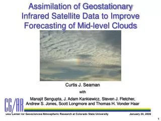
This research explores the assimilation of Geostationary Infrared Satellite Data to improve the forecasting of mid-level clouds. The study focuses on the assimilation of GOES Imager and Sounder data and the analysis of variation in decorrelation lengths and variance. The results provide insights for future improvements in cloud forecasting.

E N D
Assimilation of Geostationary Infrared Satellite Data to Improve Forecasting of Mid-level Clouds Curtis J. Seaman
Acknowledgements Advisor: Thomas H. “Tom” Vonder Haar Committee: William R. “Bill” Cotton Wayne H. Schubert Mahmood R. “Mo” Azimi (Electrical and Computer Engineering) Tomislava “Tomi” Vukicevic (University of Colorado-Boulder) Adam Kankiewicz (WindLogics, Inc.) Manajit Sengupta, Andy Jones, Steve Fletcher, Scott Longmore, Laura Fowler, Cindy Combs, Louie Grasso, John Forsythe Karll Renken, Michael Hiatt, Adam Carheden Department of Defense
Outline Introduction RAMDAS and GOES Assimilation of GOES Imager (ch. 3 & 4) Assimilation of GOES Sounder (ch. 7 & 11) Variation of decorrelation lengths and variance (background error covariance) Conclusions and Future Work
Introduction Mid-level, layered clouds (altocumulus and altostratus) are important • Cover 20-25% of the globe • Important for military, civilian aviation • Source of icing and turbulence • Obscure military targets, pilot visibility • Interfere with infrared (IR) and laser communication • Importance for climate? • Cause of blown forecasts Mid-level, layered clouds are poorly forecast • CLEX and CloudNet results • Vertically thin and most models have poor vertical resolution in mid-troposphere • Complex microphysics • Weak vertical velocity tricky to model • Models have poor moisture information (radiosonde dry bias: Soden et al. 2004) Image: Illingworth et al. (2007)
Satellite Data Assimilation • Operational forecast centers typically assimilate only cloud-free radiances • Ease, computational cost • McNally and Vespirini (1995); Garand and Hallé (1997); Ruggiero et al. (1999); McNally et al. (2000); Raymond et al. (2004); Fan and Tilley (2005) • Clouds cover 51-67% of the globe • ISCCP, CLAVR, Warren et al. (1986,1988) • Area of recent research • Marecal and Mahfouf (2002), Bauer et al. (2006), Weng et al. (2007) • Vukicevic et al. (2006) Image: NASA
Regional Atmospheric Modeling Data Assimilation System (RAMDAS) • Mesoscale 4-DVAR assimilation system designed to assimilate clear and cloudy scene VIS, IR satellite data • Forward model: RAMS • Observational operator: VISIROO • SHDOM, OPTRAN, Deeter and Evans (1998) • Developed for GOES (Imager & Sounder) • Full adjoints for VISIROO and RAMS • Includes RAMS microphysics, but not convective parameterizations
start end No Yes Regional Atmospheric Modeling Data Assimilation System (RAMDAS) Compute gradient of cost function and decide whether it is small enough yet Satellite radiance over assimilation time window Forward NWP model Forward Radiative Transfer to compute radiance from model output Update initial condition using propagated gradient of cost function. Reverse or adjoint of radiative transfer to compute adjoints Reverse or adjoint of NWP model to compute adjoints Generate forecast Greenwald et al. (2002) Zupanski et al. (2005)
The 2 Nov 2001 Altocumulus Image: RAP@UCAR
Imager Ch. 1 VIS 0.63 mm Sounder Ch. 19 VIS 0.70 mm Ch. 4 window 10.7 mm Ch. 7 window 12.0 mm Ch. 3 vapor 6.7 mm Ch. 11 vapor 7.0 mm
Experiment Set-Up 75 x 75 (6 km horiz.) x 84 (stretched-z vert.) grid centered on North Platte, NE Lateral boundaries masked to 50 x 50 x 84 to ignore boundary condition errors RAMS initialized with 00 UTC FNL (GDAS) reanalysis data 11 UTC output used to initialize RAMDAS 1145 UTC GOES observations assimilated Control Variables: p qil u,v,w rice rsnow rtotal pressure (pert. Exner function) ice-liquid potential temperature winds ice water mixing ratio snow water mixing ratio total water mixing ratio
Initial Forward Model Run Dashed = Observed Sounding; Solid = Model Sounding Initial model is poor, but we’ll use it (and get valuable results)
Experiment #1: Imager only GOES Imager channels 3 (6.7 mm) & 4 (10.7 mm)
Experiment #1: Imager only GOES Imager channels 3 (6.7 mm) & 4 (10.7 mm) Before Assimilation After Assimilation Observed Tb
Experiment #1: Imager only GOES Imager channels 3 (6.7 mm) & 4 (10.7 mm) Before assimilation After assimilation
Experiment #1: Imager only GOES Imager channels 3 (6.7 mm) & 4 (10.7 mm)
Experiment #1: Imager only GOES Imager channels 3 (6.7 mm) & 4 (10.7 mm)
Experiment #1: Imager only GOES Imager channels 3 (6.7 mm) & 4 (10.7 mm)
Experiment #1: Imager only GOES Imager channels 3 (6.7 mm) & 4 (10.7 mm) Surface wind (before) Surface wind (after)
Experiment #1: Imager only GOES Imager channels 3 (6.7 mm) & 4 (10.7 mm)
Experiment #2: Sounder only GOES Sounder channels 7 (12.02 mm) & 11 (7.02 mm)
Experiment #2: Sounder only GOES Sounder channels 7 (12.02 mm) & 11 (7.02 mm) Before Assimilation After Assimilation Observed Tb
Experiment #2: Sounder only GOES Sounder channels 7 (12.02 mm) & 11 (7.02 mm) Before assimilation After assimilation
Experiment #2: Sounder only GOES Sounder channels 7 (12.02 mm) & 11 (7.02 mm)
Experiment #2: Sounder only GOES Sounder channels 7 (12.02 mm) & 11 (7.02 mm)
Experiment #2: Sounder only GOES Sounder channels 7 (12.02 mm) & 11 (7.02 mm)
Experiment #2: Sounder only GOES Sounder channels 7 (12.02 mm) & 11 (7.02 mm) Surface wind (before) Surface wind (after)
Experiment #2: Sounder only GOES Sounder channels 7 (12.02 mm) & 11 (7.02 mm)
Decorrelation Lengths Background error covariance matrix, B, in RAMDAS based on decorrelation length and variance Assumed values of decorrelation length for each control variable shown Decorrelation lengths and variances doubled and halved
Decorrelation Lengths Increasing (decreasing) decorrelation length increases (decreases) impact of observations Variance (not shown) had little effect Note: dashed lines correspond to soundings based on default values of decorrelation length
Mid-level Cloud Decorrelation Lengths Doubled Imager Experiment Sounder Experiment
Summary • GOES Imager experiment • Cooled the surface, increased upper-tropospheric humidity • Increased fog • No closer to producing mid-level cloud • GOES Sounder experiment • Produced subsidence inversion • Cooled, humidified atmosphere near 2 km AGL • Some surface cooling • No mid-level cloud, but closer to producing one • Decorrelation lengths are important • Increasing (decreasing) decorrelation length increases (decreases) effect of observations • Variance not important • Significant innovations achieved with only one observation time • Biggest changes to temperature, dew point and winds
Conclusions • RAMDAS is designed to minimize the difference between the modeled and observed brightness temperatures • The assimilation can only modify the model state where the observations are sensitive to model variables • The mathematics doesn’t have a sense of the physics • When no cloud is present in the model, the adjoint calculates sensitivities based on having no cloud • In the GOES Imager case, ch. 4 is most sensitive to surface temperature in the absence of cloud, ch. 3 is most sensitive to upper-tropospheric humidity • GOES Sounder ch. 7 & 11 are more sensitive to low- to mid- troposphere temperature and humidity • Additional constraints are needed to ensure an appropriate physical solution
Back to the Future • Add constraints • Surface temperature • Additional cloud information • Ideal decorrelation lengths • Log-normal distributions (Fletcher and Zupanski 2007) • More channels • More case studies • CLEX-9, CLEX-10
Geostationary Operational Environmental Satellites (GOES) Theoretical Weighting Functions • Imager • Higher spatial, temporal resolution • Sounder • More channels • Experiments use window and water vapor channels • Imager ch. 3 & 4 • Sounder ch. 7 & 11 • Water vapor-only (3 & 11)
2 Nov 2001 Altocumulus from CLEX-9 • RAMS run with 100 m vertical resolution initialized with Eta 40 km reanalysis • Peak RH of 85% too low to form cloud • Radiosonde dry bias? • Will assimilation of IR water vapor radiances help?
Experiment #3: water vapor only GOES Imager ch 3 (6.7 mm) & Sounder ch 11 (7.02 mm)
Experiment #3: water vapor only GOES Imager ch 3 (6.7 mm) & Sounder ch 11 (7.02 mm) Before Assimilation After Assimilation Observed Tb
Experiment #3: water vapor only GOES Imager ch 3 (6.7 mm) & Sounder ch 11 (7.02 mm) Before assimilation After assimilation
Experiment #3: water vapor only GOES Imager ch 3 (6.7 mm) & Sounder ch 11 (7.02 mm)
Experiment #3: water vapor only GOES Imager ch 3 (6.7 mm) & Sounder ch 11 (7.02 mm)
Experiment #3: water vapor only GOES Imager ch 3 (6.7 mm) & Sounder ch 11 (7.02 mm)
Experiment #3: water vapor only GOES Imager ch 3 (6.7 mm) & Sounder ch 11 (7.02 mm) Surface wind (before) Surface wind (after)
Experiment #3: water vapor only GOES Imager ch 3 (6.7 mm) & Sounder ch 11 (7.02 mm)