Download
1 / 40
410 likes | 790 Vues
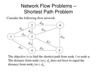
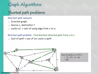
Shortest Path Problems. Directed weighted graph. Path length is sum of weights of edges on path. The vertex at which the path begins is the source vertex. The vertex at which the path ends is the destination vertex. 1. 7. Example. 8. 6. 2. 1. 3. A path from 1 to 7 . 3. 1. 16.

E N D
Shortest Path Problems Directed weighted graph. Path length is sum of weights of edges on path. The vertex at which the path begins is the source vertex. The vertex at which the path ends is the destination vertex.
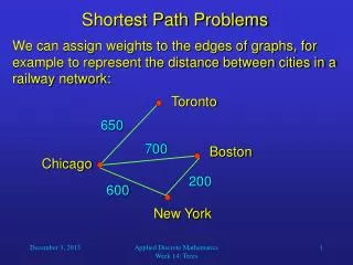
1 7 Example 8 6 2 1 3 A path from 1 to 7. 3 1 16 7 5 6 4 10 4 2 4 7 5 3 14 Path length is 14.
Example 8 6 2 1 3 Another path from 1 to 7. 3 1 16 7 5 6 4 10 4 2 4 7 5 3 14 Path length is 11.
Shortest Path Problems Single source single destination. Single source all destinations. All pairs (every vertex is a source and destination).
Single Source Single Destination Possible greedy algorithm: • Leave source vertex using cheapest/shortest edge. • Leave new vertex using cheapest edge subject to the constraint that a new vertex is reached. • Continue until destination is reached.
Greedy Shortest 1 To 7 Path 8 6 2 1 3 3 1 16 7 5 6 4 10 4 2 4 7 5 3 14 Path length is 12. Not shortest path. Algorithm doesn’t work!
Single Source All Destinations Need to generate up to n (n is number of vertices) paths (including path from source to itself). Greedy method: • Construct these up to n paths in order of increasing length. • Assume edge costs (lengths) are >= 0. • So, no path has length < 0. • First shortest path is from the source vertex to itself. The length of this path is 0.
6 1 2 1 0 9 1 3 5 4 2 1 3 10 1 3 6 5 1 3 5 11 1 3 6 7 Greedy Single Source All Destinations 8 6 2 1 3 3 1 16 7 5 6 4 10 4 2 4 7 5 3 14 Path Length
6 1 2 9 1 3 5 4 10 1 3 6 11 1 3 6 7 Greedy Single Source All Destinations Length Path • Each path (other than first) is a one edge extension of a previous path. • Next shortest path is the shortest one edge extension of an already generated shortest path. 1 0 2 1 3 1 3 5 5
Greedy Single Source All Destinations • Let d(i) (distanceFromSource(i)) be the length of a shortest one edge extension of an already generated shortest path, the one edge extension ends at vertex i. • The next shortest path is to an as yet unreached vertex for which the d() value is least. • Let p(i) (predecessor(i)) be the vertex just before vertex i on the shortest one edge extension to i.
3 2 4 7 1 [1] [2] [3] [4] [5] [6] [7] d 2 p Greedy Single Source All Destinations 8 6 2 1 3 3 1 16 7 5 6 4 10 4 2 4 7 5 3 14 0 6 2 16 - - 14 - 1 1 1 - - 1
6 5 2 1 [1] [2] [3] [4] [5] [6] [7] 1 3 d 5 10 p 3 3 Greedy Single Source All Destinations 8 6 2 1 3 3 1 16 7 5 6 4 10 4 2 4 7 5 3 14 5 0 6 2 16 - - 14 - 1 1 1 - - 1
4 7 1 [1] [2] [3] [4] [5] [6] [7] 1 3 d 9 5 10 1 3 5 p 5 3 3 Greedy Single Source All Destinations 8 6 2 1 3 3 1 16 7 5 6 4 10 4 2 4 7 5 3 14 0 6 2 16 - - 14 6 - 1 1 1 - - 1
4 1 [1] [2] [3] [4] [5] [6] [7] 1 3 d 5 10 1 3 5 p 3 3 1 2 Greedy Single Source All Destinations 8 6 2 1 3 3 1 16 7 5 6 4 10 4 2 4 7 5 3 14 0 6 2 9 - - 14 9 - 1 1 5 - - 1
7 1 [1] [2] [3] [4] [5] [6] [7] 1 3 d 5 12 1 3 5 p 3 3 4 1 2 1 3 5 4 Greedy Single Source All Destinations 8 6 2 1 3 3 1 16 7 5 6 4 10 4 2 4 7 5 3 14 10 0 6 2 9 - - 14 - 1 1 5 - - 1
7 1 3 6 [1] [2] [3] [4] [5] [6] [7] d 5 10 11 12 p 3 3 4 6 Greedy Single Source All Destinations 8 6 2 1 3 3 1 16 7 5 6 4 10 4 2 4 7 5 3 14 0 6 2 9 - - 14 - 1 1 5 - - 1
Path Length 1 0 2 1 3 1 3 5 5 1 2 6 [1] [2] [3] [4] [5] [6] [7] 9 1 3 5 4 0 6 2 9 5 - 10 - 14 12 11 - 1 1 5 3 - 3 - 4 1 6 10 1 3 6 11 1 3 6 7 Greedy Single Source All Destinations
Single Source Single Destination Terminate single source all destinations greedy algorithm as soon as shortest path to desired vertex has been generated.
Data Structures For Dijkstra’s Algorithm • The greedy single source all destinations algorithm is known as Dijkstra’s algorithm. • Implement d() and p() as 1D arrays. • Keep a linear list L of reachable vertices to which shortest path is yet to be generated. • Select and remove vertex v in L that has smallest d() value. • Update d() and p() values of vertices adjacent to v.
Complexity • O(n) to select next destination vertex. • O(out-degree) to update d() and p() values when adjacency lists are used. • O(n) to update d() and p() values when adjacency matrix is used. • Selection and update done once for each vertex to which a shortest path is found. • Total time is O(n2 + e) = O(n2).
Minimum-Cost Spanning Tree weighted connected undirected graph spanning tree cost of spanning tree is sum of edge costs find spanning tree that has minimum cost
8 10 14 1 3 5 7 3 7 12 6 4 2 2 4 6 8 9 Example • Network has 10 edges. • Spanning tree has only n - 1 = 7 edges. • Need to either select 7 edges or discard 3.
Edge Selection Greedy Strategies • Start with an n-vertex 0-edge forest. Consider edges in ascending order of cost. Select edge if it does not form a cycle together with already selected edges. • Kruskal’s method. • Start with a 1-vertex tree and grow it into an n-vertex tree by repeatedly adding a vertex and an edge. When there is a choice, add a least cost edge. • Prim’s method.
Edge Selection Greedy Strategies • Start with an n-vertex forest. Each component/tree selects a least cost edge to connect to another component/tree. Eliminate duplicate selections and possible cycles. Repeat until only 1 component/tree is left. • Sollin’s method.
Edge Rejection Greedy Strategies • Start with the connected graph. Repeatedly find a cycle and eliminate the highest cost edge on this cycle. Stop when no cycles remain. • Consider edges in descending order of cost. Eliminate an edge provided this leaves behind a connected graph.
1 3 5 7 2 4 6 8 Kruskal’s Method 8 10 14 1 3 5 7 7 3 • Start with a forest that has no edges. 12 6 4 2 2 4 6 8 9 • Consider edges in ascending order of cost. • Edge (1,2) is considered first and added to the forest.
7 3 6 4 Kruskal’s Method 8 10 14 1 3 5 7 1 3 5 7 7 3 • Edge (7,8) is considered next and added. 12 6 2 4 2 2 4 6 8 2 4 6 8 9 • Edge (3,4) is considered next and added. • Edge (5,6) is considered next and added. • Edge (2,3) is considered next and added. • Edge (1,3) is considered next and rejected because it creates a cycle.
10 14 7 3 6 4 Kruskal’s Method 8 10 14 1 3 5 7 1 3 5 7 7 3 • Edge (2,4) is considered next and rejected because it creates a cycle. 12 6 2 4 2 2 4 6 8 2 4 6 8 9 • Edge (3,5) is considered next and added. • Edge (3,6) is considered next and rejected. • Edge (5,7) is considered next and added.
10 14 7 3 6 4 Kruskal’s Method 8 10 14 1 3 5 7 1 3 5 7 7 3 • n - 1 edges have been selected and no cycle formed. • So we must have a spanning tree. • Cost is 46. • Min-cost spanning tree is unique when all edge costs are different. 12 6 2 4 2 2 4 6 8 2 4 6 8 9
10 14 1 3 5 7 7 3 6 4 2 2 4 6 8 Prim’s Method 8 10 14 1 3 5 7 7 3 • Start with any single vertex tree. 12 6 4 2 2 4 6 8 9 • Get a 2-vertex tree by adding a cheapest edge. • Get a 3-vertex tree by adding a cheapest edge. • Grow the tree one edge at a time until the tree has n - 1 edges (and hence has all n vertices).
Greedy Minimum-Cost Spanning Tree Methods • Can prove that all result in a minimum-cost spanning tree. • Prim’s method is fastest. • O(n2) using an implementation similar to that of Dijkstra’s shortest-path algorithm. • O(e + n log n) using a Fibonacci heap. • Kruskal’s uses union-find trees to run in O(n + e log e) time.
Pseudocode For Kruskal’s Method Start with an empty set T of edges. while (E is not empty && |T| != n-1) { Let (u,v) be a least-cost edge in E. E = E - {(u,v)}. // delete edge from E if ((u,v) does not create a cycle in T) Add edge (u,v) to T. } if (| T | == n-1) T is a min-cost spanning tree. else Network has no spanning tree.
Data Structures For Kruskal’s Method Edge set E. Operations are: Is E empty? Select and remove a least-cost edge. Use a min heap of edges. Initialize. O(e) time. Remove and return least-cost edge. O(log e) time.
Data Structures For Kruskal’s Method Set of selected edges T. Operations are: Does T have n - 1 edges? Does the addition of an edge (u, v) to T result in a cycle? Add an edge to T.
Data Structures For Kruskal’s Method Use an array linear list for the edges of T. Does T have n - 1 edges? Check size of linear list. O(1) time. Does the addition of an edge (u, v) to T result in a cycle? Not easy. Add an edge to T. Add at right end of linear list. O(1) time. Just use an array rather than ArrayLinearList.
1 3 5 7 7 3 6 4 2 2 4 6 8 Data Structures For Kruskal’s Method • Each component of T is a tree. • When u and v are in the same component, the addition of the edge (u,v) creates a cycle. Does the addition of an edge (u, v) to T result in a cycle? • When u and v are in the different components, the addition of the edge (u,v) does not create a cycle.
1 3 5 7 7 3 6 4 2 2 4 6 8 Data Structures For Kruskal’s Method • Each component of T is defined by the vertices in the component. • Represent each component as a set of vertices. • {1, 2, 3, 4},{5, 6},{7, 8} • Two vertices are in the same component iff they are in the same set of vertices.
1 3 5 7 7 3 6 4 2 2 4 6 8 Data Structures For Kruskal’s Method • When an edge (u, v) is added to T, the two components that have vertices u and v combine to become a single component. • In our set representation of components, the set that has vertex u and the set that has vertex v are united. • {1, 2, 3, 4} + {5, 6} => {1, 2, 3, 4, 5, 6}
1 3 5 7 2 4 6 8 • Initially,T is empty. Data Structures For Kruskal’s Method • Initial sets are: • {1} {2} {3} {4} {5} {6} {7} {8} • Does the addition of an edge (u, v) to T result in a cycle? If not, add edge to T. s1 = find(u); s2 = find(v); if (s1 != s2) union(s1, s2);
Use FastUnionFind. • Initialize. • O(n) time. • At most 2e finds and n-1 unions. • Very close to O(n + e). • Min heap operations to get edges in increasing order of cost take O(e log e). • Overall complexity of Kruskal’s method is O(n + e log e). Data Structures For Kruskal’s Method