Download
1 / 21
220 likes | 375 Vues
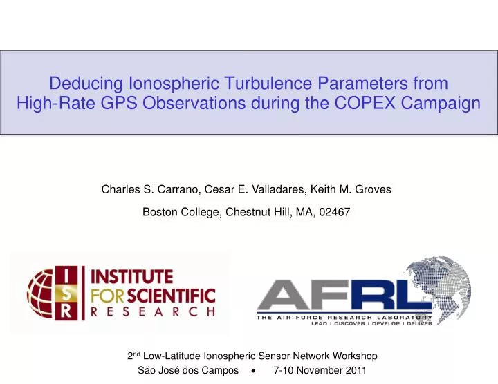
Deducing Ionospheric Turbulence Parameters from High-Rate GPS Observations during the COPEX Campaign. Charles S. Carrano, Cesar E. Valladares, Keith M. Groves Boston College, Chestnut Hill, MA, 02467.

E N D
Deducing Ionospheric Turbulence Parameters from High-Rate GPS Observations during the COPEX Campaign Charles S. Carrano, Cesar E. Valladares, Keith M. Groves Boston College, Chestnut Hill, MA, 02467 2nd Low-Latitude Ionospheric Sensor Network WorkshopSão José dos Campos 7-10 November 2011
Overview • Plasma instabilities in the equatorial ionosphere create irregularities in the electron density over a broad range of spatial scales (plasma turbulence). • These irregularities cause scintillations in the amplitude and phase of radio waves that traverse them. • Previous authors have reported on the morphology of GPS scintillations and irregularity zonal drift during the 2002 Conjugate Point Equatorial Experiment (COPEX) in Brazil. • Our focus is to use GPS observations at the three COPEX stations to characterize the turbulent ionospheric medium that produced these scintillations. • We developed a new method called Iterative Parameter Estimation for this purpose. It valid when S4 saturates due to multiple-scatter effects. This is crucial since scintillations during COPEX were too strong for weak scatter theory. • We report on the latitudinal and local time variation of turbulent intensity, spectral index, and irregularity zonal drift velocity. 2
Modeling Propagation through the Equatorial Ionosphere Transmitter We assume the plasma turbulence can be represented by a homogenous scattering layer of thickness L xp(magnetic north) These irregularities are highly elongated along Earth’s magnetic field L Propagation of radio wave through scattering layer produces a diffraction pattern on the ground Scattering Layer yp(magnetic east) z (vertical) x Receiver detects temporal fluctuations (scintillations) y Receiver t Diffraction Pattern Reception Plane Our interest is to infer characteristics of scattering layer from the time series of intensity fluctuations 4
Ionospheric Turbulence Model (Rino, 1979) • Power law model for 3D spectrum of electron density fluctuations, N: • Correlation function of phase fluctuations, R(),after passage through layer: Step 1: apply coordinate transformation to account for irregularity anisotropy Step 2: integrate through the scattering layer along the line of sight Step 3: apply Fourier Transform in the transverse plane CkL vertically integrated turbulent intensity q, q0 wavenumber, outer scale wavenumber K, modified Bessel function, Gamma function G geometry enhancement factor A,B,C propagation and B-field geometry factors • wavelength • re classical electron radius • spatial separation distance • Propagation (zenith) angle pphase spectral index (p=2) 5
The Model Intensity Spectrum (Booker and MajidiAhi, 1981) • A solution of the 4th moment equation governing intensity fluctuations following propagation of a plane wave through a thin phase-changing screen. Define Fresnel parameter: and two functions that depend on F and the phase correlation function R(): • The intensity spectrum at the reception plane is given by: • The S4 index is calculated by integrating spectrum over all wavenumbers: 6
Space-to-Time Translation (Rino, 1979) • Spatial wavenumbers translate to temporal frequencies in a model-dependent fashion: and • Effective scan velocity (Rino, 1979): where A,B,C are propagation and magnetic field geometry factors • The scan velocity (Vsx,Vsy) of the ray path through the irregularities is given by: Vpx, Vpy, Vpzare the geomagnetic north, east and down coordinates of the IPP velocity, and VD is the irregularity zonal drift velocity. 7
Iterative Parameter Estimation (IPE) • The independent variables in the ionospheric turbulence model are CkL, p, and VD All others are calculable from geometry and B field direction except the outer scale, anisotropy ratio, and layer height--we assume L0 = 10 km, a : b = 50, and Hp=350 km. • Define a metric to quantify difference between model and measured intensity spectra: Integration performed over frequency range fmin and fmax to exclude receiver noise • Solve for 3 unknown parameters iteratively using the Downhill Simplex Method 8
Two Examples of IPE Analysis Strong Scatter Example Weak Scatter Example 10
High-Rate GPS Receivers Operating During COPEX • Three sites located on nearly the same magnetic field line • Alta Floresta at dip equator • Boa Vista and Campo Grande at magnetically conjugate points, close to crests of equatorial anomaly • Three high-rate (10 Hz) Ashtech Z-CGRS receivers operated by AFRL / INPE • Data collected Oct-Dec 2002 under solar max conditions. • We present results for the evening of 1-2 Nov 2002 3
Directly Measured Parameters Vertical TEC TECU Scintillation Index Decorrelation Time b) m(sec) S4m 11
Measured and Modeled Scintillation Statistics IPE results accurately reproduce … • S4 (depth of fading) • decorrelation time, (rate of fading) Model Scintillation Index Measured Scintillation Index This is makes sense, since S4 and can be inferred from the intensity spectrum Model Decorrelation Time (sec) Previous modeling efforts have tried to reproduce either S4, or both S4 and . IPE reproduces the entire intensity spectrum Measured Decorrelation Time (sec) 12
Parameters Inferred by IPE Analysis Vertical TEC Turbulent Intensity a) TECU Log(CkL) Drift Velocity Phase Spectral Index b) VD (m/s) p 13
Phase Scintillation Parameters inferred from IPE Analysis • Spectrum of phase fluctuations: a) a) • Variance of phase fluctuations: Phase Variance Phase Spectral Strength 2(rad2) T (dB) 14
Local Time Variation at the Three COPEX Stations Turbulent Intensity Phase Spectral Strength Phase Spectral Index b) 15
Comparison with Spaced-Receiver Drift Measurements Boa Vista VHF east link (channels 3-4) VHF west link (channels 1-2) GPS spaced-receivers IPE analysis VHF spaced-receiver drift provided by Robert Livingston (SCION Associates) GPS spaced-receiver drift provided by Marcio Muella et al. [2008] Alta Floresta Campo Grande b) 16
Next Steps – Chains of Receivers from LISN Network • Apply analysis to observations from meridional chain of GPS receivers: • Can provide latitudinal and local time morphology of ionospheric turbulence responsible for scintillations at low latitudes. • Apply analysis to observations from longitudinal chain of GPS receivers: • Can provide evolution of turbulence within individual bubbles (i.e. in a coordinate system that follows the bubbles). • These GPS receivers are already operating—let’s extract the most information from them as possible! a) Longitude (deg) b) Latitude (deg) 17
Conclusions • We developed the IPE technique to characterize the turbulent ionospheric medium that produced GPS scintillations during the 2002 COPEX experiment in Brazil. • Our analysis of data collected on 1-2 Nov 2002 provides the latitudinal and local time variation of turbulent intensity, phase spectral index, and zonal drift. • The strength of turbulence tends to be largest where the TEC is largest (qualitatively) • The phase spectral index increases with local time from 2.5 to 4.5, we conjecture this is due erosion (decay) of small scale irregularities in the turbulence. • Our estimates of the zonal irregularity drift are consistent with those provided by the spaced GPS receiver technique (but our technique requires only 1 receiver) • Our drift estimates are similar at the three stations, unlike those provided by the VHF spaced-receiver technique which are larger at Campo Grande than at Boa Vista. • Next steps: Apply to LISN GPS receivers arranged in meridional/longitudinal chains • Reference: Carrano, C. S., C. E. Valladares, K. M. Groves, Latitudinal and Local Time Variation of Ionospheric Turbulence Parameters during the Conjugate Point Equatorial Experiment (COPEX) in Brazil, submitted to International Journal of Geophysics, 2011. 18
Determination of Model Parameters CkL, p, and VD Varying CkL 5.0x1034 1.0x1035 2.3x1035 5.0x1035 1.0x1036 Varying p Varying VD 75 m/s 2.5 150 m/s 3.0 212 m/s 3.6 300 m/s 3.5 4.0 400 m/s 20
Local Time Variation at the Three COPEX Stations Scintillation Index Decorrelation Time 22