Download
1 / 57
570 likes | 688 Vues
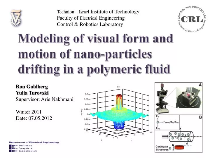
Technion – Israel Institute of Technology Faculty of Electrical Engineering Control & Robotics Laboratory. Modeling of visual form and motion of nano -particles drifting in a polymeric fluid. Ron Goldberg Yulia Turovski Supervisor: Arie Nakhmani Winter 2011 Date: 07.05.2012. Outline.

E N D
Technion – Israel InstituteofTechnologyFacultyofElectricalEngineeringControl & Robotics Laboratory Modeling of visual form and motion of nano-particles drifting in a polymeric fluid Ron Goldberg Yulia Turovski Supervisor: Arie Nakhmani Winter 2011 Date: 07.05.2012
Outline • Motivation & Goals • Previous work on the subject • System description • Modules • Example • Results • Future work
Motivation • Active and controllable drug transport • Few and isolated damaged cells • Healthy tissue unaffected • Super paramagnetic nanoplatforms • Control of platforms via magnetic field • Improve control of nanoplatforms motion • Automatic platforms characteristics and motion analysis
Goals • Automatic analysis of platforms motion and characteristics: • Static noisy background subtraction • Dynamic noise filtering • Platforms detection • Platforms modeling and reconstruction • Motion analysis • MATLAB Environment • Non real time • Short processing time (~minutes)
Input movies • Microscope generated movies • Diffraction patterns • Polymeric fluid • 15 seconds
Previous Works • Previous solution (Nakhmani et al., 2010) • Static noisy background subtraction • Dynamic noise filtering • Platforms detection • Platforms modeling and reconstruction • Motion analysis • Background subtraction: classic & advanced • Unique problem • Collection of issues • Unrelated & uncommon solutions
System Description • Noise cleaning • Static noise (background subtraction) • Dynamic noise (optional) • Particles modeling
Block Diagram Background subtraction Original movie Cleaned movie Per frame • Gaussian fitting process Marking suspicious sub frames • Circles detection Fitting errors Sub frames locations • Particles reconstruction • Sorting Algorithm Sorting results & parameters Circles parameters Reconstructed movie
Module:Background Subtraction • Based on Stauffer & GrimsonGMM algorithm • GMM – Gaussian Mixture Model • Linear superposition • Different expectations, variances and weights
Module:Background Subtraction • Stauffer & Grimson • Threshold operation • Pixel wise analysis • Mixture of Gaussians PDF • Multiple background objects • Continuously updating model’s parameters
Module:Background Subtraction • Improved Implementation • External source • Dynamic number of Gaussians • Results & run time improved
Module:Background Subtraction • Improvement • Merging regular and reversed movies • Learning process • Later frames better cleaned • Linear weight:
Background Subtraction:Example Original frame Cleaned frame
Module:Particles Detection I • Particles’ diffraction patterns • Theoretically: Bessel functions • Practically: Bessel functions & Gaussians • Initial detection • Sub frames • Gaussian fitting • Revaluation error
Module:Particles Detection I • Gaussian fitting • Least squares • Linearization of Gaussian model • Pseudo Inverse • Mean Square Error • Normalized to revaluated amplitude
Module:Particles Detection I • Improved disadvantages • Sensitivity to zeros & low intensities • Saturation • Pseudo inverse • Perfect revaluation for ideal Gaussians • Impressive revaluation & detection capabilities • Excellent reliability • Thousands sub frames per frame • Numbered error messages
Module:Particles Detection I • Particles detection in frames • Uniform sub frames ( ) • Overlap (50% in each axis) • Filtering out hopeless sub frames • Negative revaluation error image
Particles Detection I:Example (III) Frame 1 Frame 2 Fitting error - frame 2 Fitting error - frame 1
Module:Particles Detection II • Sub frames matching • For circle detection • Sub frames depend on suspicious areas • Revaluation error based algorithm • Clear distinction • Suspicious areas • Size of sub frames
Module:Particles Detection II • Chosen method • Lower threshold • Square sub frame • Exponential formula for area:
Module:Particles Detection II • : Revaluation error • : Lower threshold • : Sub frame’s maximum area • : Sub frame’s minimum area • : Curvature of exponential function • , descending function • Spans sub frames sizes
Particles Detection II:Example Frame 1 Frame 2 Calculated frames of frame 2 Calculated frames of frame 1
Module:Particles Detection II • Good compatibility with particles • Size • Location • Multiple sub frames dealt by sorting algorithm
Module:Circles Detection • Centers and radii • Basis for particles modeling • Popular problem • Many circles detection algorithms exist • Chosen solution from external source • Chosen algorithm • Gray scale input images • Based on circular Hough transform
Module:Circles Detection • Circular Hough transform • Method for detecting shapes in images • Basic transform detects straight lines • Generalization to circles & ellipses • Further Generalization to any parametric shape • Shapes detected in parameter space • Chosen algorithm enables control of: • Allowed asymmetry • Sensitivity to concentric circles
Module:Circles Detection • Suitable solution • Revaluation error based detection • Sub frames matching for suspicious areas • On each sub frame • Chosen algorithm is performed • Uniform parameters set • Circles data is accumulated
Circles Detection:Example Frame 1 Frame 2
Module:Sorting Algorithm • Overlap causes need to cross data from different structures Reconstructed frame Original frame
Module:Sorting Algorithm • Sorts to Gaussians and Besselians • Considers all circles detected • Handles structures separately • Each structure can contain several particles • Initial & temporary sorting • Crosses data from different structures • Filtering out resembling circles • Final sorting
Module:Sorting Algorithm • Determines equivalent centers for Besselians • Based on two largest radii • Linear weight • Bigger weight for larger circle
Sorting Algorithm:Example (I) Circles frame Sorted circles frame
Sorting Algorithm:Example (II) Circles frame Sorted circles frame
Sorting Algorithm:Example (II) Reconstructed frame Original frame
Sorting Algorithm:Example (III) Frame 1 Frame 2
Module:Particles Reconstruction • Based on sorted circles • Gaussian particles • Least squares Gaussian fitting • Same algorithm used for particles detection • Selected sub frames • Sub frames’ sizes determined by circles data
Module:Particles Reconstruction • Besselian particles • Sub frames’ sizes determined by circles data • Besselian formula: • Needed parameters: &
Module:Particles Reconstruction • : • Zeros of Besselian known • Detected circles are zero contours • computed using smallest circle’s radius • : • Common Besselians: • Truncated main lobe • Just one ring
Module:Particles Reconstruction • : • Reconstruction based on first ring: • Analytic function’s mean known • First ring’s mean computed • Comparison of both gives Analytic Function First ring
Particles Reconstruction:Example (I) Original particle Detected circles Original particle’s first ring Reconstructed particle
Particles Reconstruction:Example (II) Reconstructed frame Original frame
Results • System’s products • Reconstructed movie • Circles’ data • Limited quantitative analysis • Qualitative analysis • Satisfactory results • Unsatisfactory results
Quantitative analysis Frame 1 Frame 2
Quantitative analysis Frame 1 Frame 2 Frame 1 reconstructed Frame 2 reconstructed
Quantitative analysis • Centers of mass • Manual radii calculation • Frame 1: • 16 particles • 9 correct detections • 7 misses • 6 false detections • Mean distance: 1.32 • Distance standard deviation: 0.96 • Frame 2: • 13 particles • 12 correct detections • 1 miss • 1 false detection • Mean distance: 2.75 • Distance standard deviation: 2.16
Qualitative analysis Original Frame • Satisfactory results Cleaned Frame Reconstructed Frame
Qualitative analysis • Impressive reconstruction • Conspicuous & small particles • Inconspicuous & weak particles • Asymmetric & imperfect particles • Particles in noisy environment • Reconstruction algorithm corrects detection algorithm’s faults.