Download
1 / 26
260 likes | 357 Vues
J. Zallat , S. Faisan, M. Karnoukian , C. Heinrich, M. Torzynski , A. Lallement. self- calibrating polarimeters and advanced image- like data reconstruction/ processing algorithms. Polarization imaging. Access specific properties of objects and media. Application dependent .

E N D
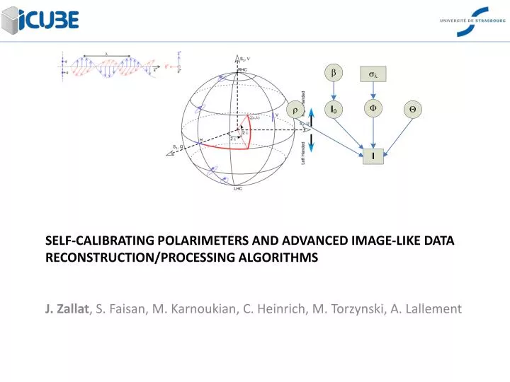
J. Zallat, S. Faisan, M. Karnoukian, C. Heinrich, M. Torzynski, A. Lallement self-calibratingpolarimeters and advanced image-like data reconstruction/processingalgorithms
Polarizationimaging Access specificproperties of objects and media.Application dependent. Distributedmeasurements of polarizationparameters Experimentaldevelopments • Polarimeters • Calibration • Authenticate acquisitions • Robustness Physicalimagingmodality Observation model Measuredquatities (radiances) Physicalquantities Stokes - Mueller • Theoreticaldevelopments • Model inversion • Polarizationalgebra • Signal/Image processing • Physicalinterpretation • Relevant display
Polarization imaging consists in an indirect distributed measurement of polarization properties of light. Observables that lead to desired physical quantities are “noisy”. • A multi-component information is attached to each pixel of the image. • Simple observation model that amplify noise when classical pseudo-inverse approach is used. • Classical analysis methods are pixel-wise oriented.
SNR = 20 dB: 54% des pixels sont non admissibles! SNR = 10 dB: 57% des pixels sont non admissibles!
Application: données synthétiques True Mueller Intensities Betterapproach Naïve inversion
Polarimetric Calibration Spectral calibration of a polarimeter: RWP
Spectral calibration of a polarimeter: LCVR Classical LCVR - PSA L2 P L1 New LCVR – PSA Differential PSA L2 P L1 HW
Spectral calibration of a polarimeter: Stability L2 P L1 HW P’
Verywellconditionedpolarimeter. • The PSA is very stable, no necessity to recalibrate over a long period! • It is used now to construct a full field Mueller imaging polarimeter dedicated to small animals tissues studies.
Data reduction For each pixel location (s), we have For each class: To account for non uniform illumination, a gaussian mixture densityisused to model:
M1 = [ 1.0000 0.0044 -0.0243 0.0488 -0.0166 0.3616 -0.0552 -0.1671 -0.0417 -0.0122 0.2991 -0.3169 -0.0077 0.1675 0.2551 0.2231 ] M2 = [ 1.0000 0.0249 0.0101 0.0014 0.0135 0.9011 -0.2090 -0.3613 0.0115 -0.1105 0.6968 -0.6963 0.0179 0.4028 0.6741 0.6083 ] M3 = [ 1.0000 -0.3102 -0.5205 0.7648 -0.4711 0.1691 0.2453 -0.3734 -0.8678 0.2605 0.4672 -0.6785 -0.0083 0.0112 0.0224 0.0052 ] M4 = [ 1.0000 0.0053 0.0075 0.0052 0.0012 0.8993 -0.2341 -0.3621 0.0042 -0.0898 0.7110 -0.6907 0.0069 0.4224 0.6565 0.6171 ] M5 = [ 1.0000 0.4296 0.4694 -0.7280 0.5207 0.2426 0.2414 -0.3865 0.8273 0.3613 0.4156 -0.6273 0.0013 0.0042 0.0285 0.0002 ]
Conclusion Efficient imagingpolarimetry: Balance between system complexity and ad hoc data reductionalgorithms. To find an information, it must bepresent in the data: The most informative data are the « raw data ».