Download
1 / 52
520 likes | 624 Vues
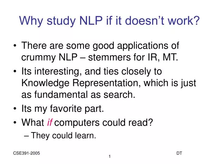
Why study NLP if it doesn’t work?. There are some good applications of crummy NLP – stemmers for IR, MT. Its interesting, and ties closely to Knowledge Representation, which is just as fundamental as search. Its my favorite part. What if computers could read? They could learn.

E N D
Why study NLP if it doesn’t work? • There are some good applications of crummy NLP – stemmers for IR, MT. • Its interesting, and ties closely to Knowledge Representation, which is just as fundamental as search. • Its my favorite part. • What if computers could read? • They could learn. DT
Introduction to Learning • Learning is the ability to improve behavior based on experience. • Components of a Learning Problem • task - behavior being improved • data - experiences being used to improve performance • measure of improvement- e.g., accuracy in prediction, speed, coverage • background knowledge - bias on what can be learned DT
Choosing a Representation for Learning • The richer the representation, the more useful for subsequent problem solving • The richer the representation, the more difficult it is to learn • Alternative representations: • Bayesian classifiers • Decision Trees • Neural Nets DT
Feedback to the Learner • Supervised learning: Learner told immediately whether response behavior was appropriate (training set) • Unsupervised learning: No classifications are given; the learner has to discover regularities and categories in the data for itself. • Reinforcement learning: Feedback occurs after a sequence of actions DT
Measuring Success • Training set, test set • The measure of success is not how well the agent performs on the training examples, but how well it performs for new examples. DT
Learning as Search • Given a representation and a bias, • Learning is search through the space of possible representations, looking for the one(s) that best fit(s) the data, given the bias. • These search spaces are typically prohibitively large for systematic search. Use hill climbing. • A learning algorithm is thus made up of • search space • an evaluation function • search method DT
Decision Trees: Chap 18.1-18.3 • Introduction • Definition • Using Decision Trees • Building decision trees • recursive partitioning • information gain ratio • Overfitting • Pruning • When are Decision trees useful DT
Introduction • Goal: Categorization • Given an event, predict its category. • Who won a given ball game? • How should we file a given e-mail? • What word sense was intended for a given occurrence of a word? • Event = list of features. • Ball game: Which players were on offense? • E-mail: who sent the message? • Disambiguation: what was the preceding word? DT
Introduction, cont. • Use a decision tree to predict categories for new events. • Use training data to build the decision tree. New event Training events and categories Decision Tree Category DT
Decision Trees • A decision tree is a tree where • each node is labeled with a feature • each arc of an interior node is labeled with a value for that feature. • each leaf is labeled with a category location away home goalie weather dry wet Jane Bob dry win time weather lose 5pm wet 3pm win lose lose win 4pm DT win
Word Sense Disambiguation • Given an occurrence of a word, decide which sense, or meaning, was intended. • Example, run • run1: move swiftly ( I ran to the store.) • run2: operate (I run a store.) • run3: flow (Water runs from the spring.) • run4: length of torn stitches (Her stockings had a run.) DT
Word Sense Disambiguation • Categories • Use word sense labels (run1, run2, etc.) • Features – describe context of word • near(w) : is the given word near word w? • pos: word’s part of speech • left(w): is word immediately preceded by w? • etc. DT
Using a decision Tree • Given an event (=list of feature values): • Start at the root. • At each interior node, follow the outgoing arc for the feature value that matches our event • When we reach a leaf node, return its category. run4 pos verb noun “I saw John run a race by a river.” near(stocking) near(race) yes no yes no run1 near(river) yes run3 4pm DT
Building Decision TreesAutomatically - Learning • Representation is a decision tree. • Bias (built-in preference) is towards “simple” decision trees. • Search through the space of decision trees, from simple trees to more complex ones. DT
Ex 1: Learning When User will Read Article Example User Action Author Thread Length e1 skips known new long e2 reads unknown new short e3 skips unknown follow-up long e4 skips known follow-up long e5 reads known new short e6 skips known follow-up long e7 skips unknown follow-up short e8 reads unknown new short e9 skips known follow-up long e10 skips known new long e11 skips unknown follow-up short e12 skips known new long e13 reads known follow-up short e14 reads known new short DT
Ex 1: Learning When User will Read Article Example User Action Author Thread Length e15 reads known new short e16 reads known follow-up short e17 reads known new short e18 reads unknown new short 9 skips, 9 reads DT
Characterizing When User Reads Articles thread author new follow-up unknown known author thread follow-up unknown new known Decision Tree Learning: Supervised learning from a set of examples. DT
Example User Action Author Thread Length e1 skips known new long e4 skips known follow-up long e5 reads known new short e6 skips known follow-up long e9 skips known follow-up long e10 skips known new long e12 skips known new long e13 reads known follow-up short e14 reads known new short e15 reads known new short e16 reads known follow-up short e17 reads known new short Learning when the user reads an article: Author = known? 6 skips, 6 reads DT
Learning when the user reads an article: Thread = new? Example User Action Author Thread Length e1 skips known new long e2 reads unknown new short e5 reads known new short e8 reads unknown new short e10 skips known new long e12 skips known new long e14 reads known new short e15 reads known new short e17 reads known new short e18 reads unknown new short 3 skips, 7 reads DT
Learning when the user reads an article: Length = long? Example User Action Author Thread Length e1 skips known new long e3 skips unknown follow-up long e4 skips known follow-up long e6 skips known follow-up long e9 skips known follow-up long e10 skips known new long e12 skips known new long 7 skips, 0 read DT
Learning Decision Trees • A decision tree is a tree whose • non-leaf nodes are labeled with • attributes (features) • - arcs from a node labeled with attribute A are • labeled with possible values of A • - leaf nodes (leaves) are labeled with classifications • Once a decision tree is learned, new examples can be classified by filtering them down the tree. • Training data is often consistent with several different • decision trees. DT
Searching for a Good DTree • The input is a target attribute (the goal), a set of examples, and a set of attributes. • Stop tree building if all examples belong to the same class. • Otherwise, choose an attribute to split on. For each value of the attribute, build a subtree for the examples with this value. • It should be simple. • Occam’s Razor – simple models generalize better • In simpler decision trees, each node is based on more data (on average). → More reliable. • But, maximum entropy bias is towards “more complexity”! DT
Searching for a Good DTree • The input is a target attribute (the goal), a set of examples, and a set of attributes. • Stop tree building if all examples belong to the same class. • Otherwise, choose an attribute to split on. How do you choose? Information gain. For each value of the attribute, build a subtree for the examples with this value. • It should be simple. • Occam’s Razor – simple models generalize better • In simpler decision trees, each node is based on more data (on average). → More reliable. • But, maximum entropy bias is towards “more complexity”! DT
Information Theory To distinguish 4 items, need 2bits? 00,01,10,11 In general, distinguish n items with log2n bits. But, with probabilities….. p(a) = 1/2, p(b) = 1/4, p(c) = 1/8, p(d) = 1/8 a 0b 10c 110 d 111 aacabbda 00110010101110(14 bits < 16 bits) p(a) *1+ p(b) *2 + p(c) *3 + p(d)*3 1/2+ 2/4 + 3/8 + 3/8 = 1 ¾ bits(instead of 2 bits) -log2 p(x) bits DT
Information Theory -log2 p(x) bits As the probabilities get smaller, the -logs get bigger. The higher the probability of the most probable item, the smaller the average number of bits DT
I - Information contentaka H • Identifying a member of a distribution: • The expected # of bits to describe a distribution given evidence e: DT
Information gain Given a test that distinguishes a from ¬a: where I(true) is bits needed before the test, and you want to know the difference between that and bits needed after the test expected entropy of a feature DT
Expected entropy of thread=new(aka NThread = true) NThread, (3 skips, 7 reads), need I(NThread) I(Nthread) = - 0.3 x log2 0.3 - 0.7 x log2 0.7 = 0.881 DT
Expected entropy of thread=followup(aka NThread = false) ¬NThread, (6 skips, 2 reads), need I(¬NThread) - 0.75 x log2 0.75 - 0.25 x log2 0.25 = 0.811 DT
Information gain of thread, length • I(NThread)= 0.881, I(¬Nthread) = .811 1.0 – ((10/18) x 0.881 + (8/18) x 0.811)) = 0.150 1.0 –((7/18) x 0 + (11/18) x 0.684)) = 0.582 Longlength,¬ Longlength, DT
Using Decision Tree Learning in Practice • Attributes can have more than two values, complicating the tree and tree-building • Attributes may be inadequate for representing the data. May want to return probabilities at leaves. • Which attribute to split on isn’t defined. Usually bias towards smallest tree. • Overfitting is a problem. DT
Overfitting • Decision tree may encode idiosyncrasies of training data – how much do we trust a leaf based on one training sample? yes no yes no yes no no no yes yes yes no yes run1 run2 run3 run4 run1 run6 run7 run8 DT
Overfitting • Fully consistent decision trees tend to overgeneralize • Especially if the decision tree is big • Or if there is not much training data • Trade-off full consistency for compactness • Larger decision trees can be more consistent • Smaller decision trees generalize better DT
Handling Overfitting • One can restrict splitting, so that split only when split is “useful”. • Threshold for max(information gain) = θ • Threshold for # of samples = κ • One can allow unrestricted splitting and prune the resulting tree where it makes unwarranted distinctions. DT
Pruning • We can reduce overfitting by reducing the size of the decision tree • Create the complete decision tree • Discard any unreliable leaves • Repeat until the decision tree is compact enough • Which leaves are unreliable? • low counts? • When should we stop? • no more unreliable leaves? DT
Held-Out Data • How can we tell if we’re overfitting? • Use a subset of the training data to train the model (the “training set”) • Use the rest of the training data to test for overfitting (the “held-out set” or “development set”) DT
Held-out Data • Pruning with held-out data • Create the complete decision tree from training data • Test the performance on the held-out set • For each leaf • Test the performance of the decision tree on the held-out set without that leaf. • If the performance improves discard the leaf. • Repeat until no more leaves are discarded DT
When are decision trees useful? • Disadvantages of decision trees • Problems with sparse data and overfitting • Pruning helps, but doesn’t completely solve • Don’t directly combine information about different features • Advantages of decision trees • Fast • Easy to interpret • Helps us understand what’s important about a new domain • We can explain why the decision tree makes decisions DT
Choosing a Representation for Learning • The richer the representation, the more useful for subsequent problem solving • The richer the representation, the more difficult it is to learn • Alternative representations: • Bayesian classifiers • Decision Trees • Neural Nets DT
Modeling thinking? • Do decision trees model thinking? • Do decision trees work the way our brain does? • Do airplanes fly the way birds do? • What would be closer to our brain? DT
Neural Networks • Representations inspired by neurons and their connections in the brain. • Artificial neurons (units) have inputs and an output that can be connected to the inputs of other units. • The output of a unit is a parameterized non-linear function of its inputs. • Learning occurs by adjusting parameters to fit data • Neural networks can represent an approximation to any function. (like Dtrees) DT
Neural net for “news” example Input units hidden units output unit known new short home DT
Pseudo-code for “news” net • predicted_prob(Obj, reads, V) • prob(Obj,h1, I1), • prob(Obj,h2, I2), • V is f(w0 + w1 * I1 + w2 * I2). • Output is in the range 0 to 1 DT
Pseudo-code for “news” net • predicted_prop(Obj, h1, V1) • prop(Obj,known, I1), • prop(Obj,new, I2), • prop(Obj,short, I3), • prop(Obj,home, I4), • V1 is f(w3 + w4 * I1 + w5 * I2 + w6 * I3 + w7 * I4). DT
Pseudo-code for “news” net • predicted_prop(Obj, h2, V2) • prop(Obj,known, I1), • prop(Obj,new, I2), • prop(Obj,short, I3), • prop(Obj,home, I4), • V2 is f(w8 + w9 * I1 + w10 * I2 + w11 * I3 + w12 * I4). • The trick is learning the values for w’s • Back-propogation (start with random values, • Compare predicted output w/ observed output & backup) DT
Neural Net Learning • Aim of neural net learning: given a set of examples, find parameter settings that minimize the error. • Back-propagation learning is gradient descent search through parameter space to minimize the sum-of-squares error. DT
Back propagation Learning • Inputs • a network, with units and their connections • stopping criterion • learning rate (constant of proportionality for parameter modification) • initial values for the parameters • set of classified training data • Output: Updated values for the parameters DT
“Backprop” algorithm • Repeat • evaluate the network on each example, given the parameter settings • determine the derivative of the error for each parameter • change the parameter in proportion to its derivative • until the stopping criterion is met. • May take hundreds/thousands of iterations DT
Examples of Multi-layer Net Learning • NETtalk (Sejnowski & Rosenberg 1987) • - 29 input units per position (encoding A-Z , . <space>) • - 26 output units (corresponding to 21 articulatory • features, 5 features of stress or syllable boundary) • - 80 hidden units • - 18,629 connections whose weight had to be learned • - training data: 7 character window, from which • pronunciation of middle character to be learned. • After training on 500 examples (100 passes through the • training data), NETtalk could correctly pronounce 60% • of the test data. DT