Download
1 / 92
1.07k likes | 1.57k Vues
CHAPTER 10. Systems of Linear Differential Equations. Contents. 10.1 Preliminary Theory 10.2 Homogeneous Linear Systems 10.3 Solution by Diagonalization 10.4 Nonhomogeneous Linear Systems 10.5 Matrix Exponential. 10.1 Preliminary Theory.

E N D
CHAPTER 10 Systems of Linear Differential Equations
Contents • 10.1 Preliminary Theory • 10.2 Homogeneous Linear Systems • 10.3 Solution by Diagonalization • 10.4 Nonhomogeneous Linear Systems • 10.5 Matrix Exponential
10.1 Preliminary Theory • IntroductionRecall that in Sec 3.11, we have the following system of linear DEs: (1)
Linear Systems • When (2) is linear, we have the normal form as (3)
Matrix Form of a Linear Systems • If we letthen (3) becomes (4)If it is homogeneous, (5)
Example 1 (a) If , the matrix form of is
DEFINITION 10.1 Solution Vector A solution vector on an interval I is any column matrix whose entries are differentiable functions satisfying (4) on the interval.
Example 2 • Verify that on (−, ) are solutions of (6)
Example 2 (2) SolutionFromwe have
Initial Value Problem (IVP) • Let Then the problem with X(t0) = X0 (7)is an IVP.
THEOREM 10.1 Let the entries of A(t) and F(t) be continuous functions on a common interval I that contains t0, Then there exists a unique solution of (7) on I. Existence of a Unique Solution THEOREM 10.2 Let X1, X2,…, Xk be a set of solutions of the homogeneous system (5) on I, thenX = c1X1 + c2X2 + … + ckXkis also a solution on I. Superposition Principles
Example 3 • Please verify that are solutions of (8)
Example 3 (2) then is also a solution.
DEFINITION 10.2 Let X1, X2, …, Xk be a set of solution vectors of the homogeneous system (5) in an interval I. We say the set is linear dependent in the interval if there exist constants c1, c2, …, ck, not all zero, such that c1X1 + c2X2 + … + ckXk = 0 for every t in the interval. If the set of vectors is not linearly dependent on the interval, it is said to be linearly independent. Linear Dependence/Independence
THEOREM 10.3 Letbe n solution vectors of the homogeneous system (5) on an interval I. Then the set of solution vectors is linearly Independent on I if and only if the Wronskian Criterion for Linearly Independent Solution
(continued) THEOREM 10.3 (9)for every t in the interval. Criterion for Linearly Independent Solution
(continued) If are linearly dependent on I, then W=0 at every point of I. If are linearly independent on I, then W 0 at every point of I. Criterion for Linearly Independent Solution
Example 4 • We saw thatare solutions of (6). Since they are linearly independent for all real t.
DEFINITION 10.3 Any set of n linearly independent solution vectors X1, X2, …, Xnof the homogeneous system (5) on an Interval I is said to be a fundamental set of solutions on the interval. Fundamental Set of Solution
THEOREM 10.4 There exists a fundamental set of solutions for the homogeneous system (5) on an interval I. Existence of a Fundamental Set THEOREM 10.5 Let X1, X2, …, Xn be a fundamental set of solutions of the homogeneous system (5) on an interval I. Then the general solution of the system in the interval is X = c1X1 + c2X2 + … + cnXnwhere the ci, i = 1, 2,…, n are arbitrary constants. General Solution—Homogeneous Systems
Example 5 • We saw thatare linearly independent solutions of (6) on (−, ). Hence they form a fundamental set of solutions. Then general solutions is then (10)
Example 6 • Consider the vectors
Example 6 (2) • Their Wronskian is
Example 6 (2) • Then the general solution is
THEOREM 10.6 General Solution—Nonhomogeneous Systems Let Xp be a given solution of the nonhomogeneous system (4) on the interval I, and let Xc = c1X1 + c2X2 + … + cnXndenote the general solution on the same interval of the associated homogeneous system (5). Then the general solution of the nonhomogeneous system on the interval is X = Xc + Xp. The general solution Xc of the homogeneous system (5) is called the complementary function of the nonhomogeneous system (4).
Example 7 The vector is a particular solution of (11)on (−, ). In Example 5, we saw the solution of isThus the general solution of (11) on (−, ) is
10.2 Homogeneous Linear Systems • A QuestionWe are asked whether we can always find a solution of the form (1)for the homogeneous linear first-order system (2)
Eigenvalues and Eigenvectors • If (1) is a solution of (2), then X = Ket then (2) becomes Ket = AKet . Thus we have AK = K or AK – K = 0. Since K = IK, we have (A – I)K = 0 (3) The equation (3) is equivalent to
If we want to find a nontrivial solution X, we must have det(A – I) = 0The above discussions are similar to eigenvalues and eigenvectors of matrices.
8.8 The Eigenvalue Problems DEFINITION 8.13 Let A be n n matrix. A number is said to be an eigenvalue of A if there exists a nonzero solution vector K of AK = K(1)The solution vector K is said to be an eigenvector corresponding to the eigenvalue . Eigenvalues and Eigenvectors
Procedure for finding a solution Step 1: Determine the eigenvalue . Step 2: Determine the associated eigenvector by solving AK= K Step 3: Form a solution K .
THEOREM 10.7 Let 1, 2,…, n be n distinct eigenvalues of the matrix A of (2), and let K1, K2,…, Kn be the corresponding eigenvectors. Then the general solution of (2) is General Solution—Homogeneous Systems
THEOREM Let 1, 2,…, n be n distinct eigenvalues of the matrix A of (2), and let K1, K2,…, Kn be the corresponding eigenvectors. Then K1, K2,…, Kn are linearly Independent.
Example 1 Solve (4) Solutionwe have 1 = −1, 2 = 4.
Example 1 (2) For 1 = −1, we have 3k1 + 3k2 = 0 2k1 + 2k2 = 0Thus k1 = – k2. When k2 = –1, then For 1 = 4, we have −2k1 + 3k2 = 0 2k1 − 2k2 = 0Thus k1 = 3k2/2. When k2 = 2, then
Example 1 (3) We have and the solution is (5)
Example 2 Solve (6) Solution
Example 2 (2) • For 1 = −3, we have Thus k1 = k3, k2 = 0. When k3 = 1, then (7)
Example 2 (3) • For 2 = −4, we have Thus k1 = 10k3, k2 = − k3. When k3 = 1, then (8)
Example 2 (4) • For 3 = 5, we have Then (9)
Example 2 (5) • Thus
Example 3: Repeated Eigenvalues Solve Solution
Example 3 (2) (repeated eigenvalue is complete) • We have – ( + 1)2(– 5) = 0, then 1 = 2 = – 1,3 = 5.For 1 = – 1,k1 – k2 + k3 = 0 or k1 = k2 – k3. Choosing k2 = 1, k3 = 0 and k2 = 1, k3 = 1, in turn we have k1 = 1 and k1 = 0.
Example 3 (3) • Thus the two linearly independent eigenvectors areFor 3 = 5,
Example 3 (4) • Implies k1 = k3 and k2 = – k3. Choosing k3 = 1, then k1 = 1, k2 = –1, thusThen the general solution is
DEFINITION 7.7 A set of vectors {x1, x2, …, xn} is said to be linearly independent, if the only constants satisfying k1x1 + k2x2 + …+ knxn = 0 (3) are k1=k2 = … = kn = 0. If the set of vectors is not linearly independent, it is linearly dependent. Linear Independence
Repeated eigenvalue is defective • Suppose 1 is of multiplicity 2 and there is only one eigenvector. A second solution will be of the form (12)Thus X = AX becomeswe have (13) (14)
Example 4 Solve SolutionFirst solve det (A – I) = 0 = ( + 3)2, = -3, -3, and then we get the first solutionLet