Download
1 / 23
230 likes | 236 Vues
This lecture explores the challenges and techniques in designing parallel algorithms for sparse matrix operations, including latency hiding, tiling for coalesced reads, and maximizing occupancy. The lecture also covers topics such as breadth-first graph traversals, sieves, and N-body problems.

E N D
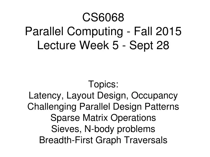
CS6068 Parallel Computing - Fall 2015Lecture Week 5 - Sept 28Topics:Latency, Layout Design, OccupancyChallenging Parallel Design PatternsSparse Matrix OperationsSieves, N-body problemsBreadth-First Graph Traversals
Latency versus Bandwidth • Latency is time to complete task – eg load memory and do FLOP • Bandwidth is throughput or number of tasks per unit time – eg peak global to shared memory load rate, or graphic frames per sec • GPUs optimize for Bandwidth – employ techniques to hide latency • Reasons Latency lags Bandwidth over time • Moore’s Law favors Bandwidth over Latency • Smaller, faster transistors but communicate over longer wires, which limits Latency • Increasing Bandwidth with queues hurts Latency
Techniques for Performance • Hiding Latency and Little’s Law • Number useful Bytes delivered = Average Latency x Bandwidth • Tiling for coalesced reads and utilization of shared memory • Synchthreads barriers and block density • Occupancy – latency hiding achieved by maximize the number of active blocks per SM
Considerations For Sizing Tiles: • Need to make sure that: • Tiles are large enough to get speedups by lowering average latency • Tiles are small enough so we can fit into the shared/register memory limits and • Use many tiles so that groups of thread blocks running on SM fill memory bus
Sizing Tiles • How Big Should We Make a Tile? • If we choose a larger tile, does that mean more or less total main memory bandwidth? • If choose larger tile, does that mean easier or harder to make use of shared memory? • 3. If choose larger tile, does that mean we wait longer or shorter to synchronize? • 4. If choose larger tile, does that mean we can more easily hide latency better?
Warps and Stalls • A grid is composed of blocks which are completely independent. • A block is composed of threads which can communicate within their own block • Instructions are issued within an SM on a per warp basis -- and generally 32 threads form a warp • If an operand is not ready the warp will stall • Context switch between warps when stalled, and for performance context switch must be very fast
Fast Context Switching • Registers and shared memory are allocated for an entire block, as long as that block is active • Once a block is active it will stay active until all threads in that block have completed • Context switching is very fast because registers and shared memory do not need to be saved and restored • Goal: Have enough transactions in flight to saturate the memory bus • Latency is better hidden when there are more transactions in flight.
OccupancyOccupancy is an easy, if somewhat imprecise, measure of how well we have saturated the memory pipeline for latency hiding.In a Cuda Program we measure occupancy as follows: Ratio of #Active Warps to #Maximum Active WarpsResources are allocated for the entire block and are thus potential occupancy limiters: Register usage, Shared memory usage, Block size
Occupancy Examples • Fermi Streaming Multiprocessor SM specs: • 1536 threads (Max Threads) = • 48 active warps of 32 threads per warp • Example 1: Suppose SM has 48K shared memory • Program Kernel uses 32 bytes of shared memory per thread • 48K/32 = 1536, so we can actively schedule 1536 threads or 48 warps • Max Occupancy limit = 1 • Example 2: Suppose SM has 16K shared memory • Program Kernel uses 32 bytes of shared memory per thread • 16K/32 = 512, so we can actively schedule only 512 threads per block or 16 warps • Max occupancy limit =.3333 Cuda Toolkit includes: • occupancy_calculator.xls
A Classic Problem: Dense N-Body Compute an NxN matrix of Force vectors • N objects – each with own parameters, 3D-location, mass, charge, etc. • Goal: Compute N^2 Source/Dest Forces • Solution 1: partition threads using PxP tiles • Q: how to minimize average latency • ratio of global versus shared memory fetches • Solution 2: partition space using P threads using spacial locality • Privatization principle: avoid write conflicts • Impact of Partition on Bandwidth, Shared Memory, and Load Imbalance ???
Sparse Matrix Dense Vector Products • A format for sparse matrices using 3 dense vectors: • Compressed Sparse Row CSR format • Value = nonzero data one array • Column= identifies column for each value • Rowptr= pointers to location of each 1st data in each row
Segmented Scan • Sparse Matrix multiplication requires modified scan, called a segmented scan in which there is special symbol indicating segments within array, and scan are done per segment • Apply scan operation to segments independently • Reduces to ordinary scan where we treat segment symbol as an annihilation value • Work an example using both inclusive and exclusive scans.
Dealing with Sparse Matrices • Apply dense format CSR • Apply segmented Scan Operations • Granularity considerations • Thread per Row vs Thread per Element • Load imbalance • Hybrid Approach?
Sieve of Eratosthenes: Sequential Algorithm A Classic Iterative Refinement: Sieve of Eratosthenes 2 2 3 3 4 4 5 5 6 6 7 7 8 8 9 9 10 10 11 12 12 13 14 14 15 15 16 16 17 18 18 19 20 20 21 21 22 22 23 24 24 25 25 26 26 27 27 28 28 29 30 30 31 32 32 33 33 34 34 35 35 36 36 37 38 38 39 39 40 40 41 42 42 43 44 44 45 45 46 46 47 48 48 49 49 50 50 51 51 52 52 53 54 54 55 55 56 56 57 57 58 58 59 60 60 61
Sieve of E - Python code def findSmallest(primes, p): #helper function for i in range(p, len(primes)): #finds smallest prime after p if primes[i] == 1: return i def sieve(n): #return num primes less than n primes = numpy.ones((n+1,), dtype=numpy.int) primes[0]=primes[1]=0 k=2 while (k*k <= n): mult= k*k while mult <= n: primes[mult] = 0 mult = mult + k k = findSmallest(primes,k+1) return sum(primes)
>>>import time, numpy for x in range(15,27): st=time.clock(); s=sieve(2**x); fin=time.clock() print x, s, fin-st x sum time 15 3512 0.04 16 6542 0.1 17 12251 0.17 18 23000 0.35 19 43390 0.71 20 82025 1.44 21 155611 2.94 22 295947 5.89 23 564163 11.93 24 1077871 24.67 25 2063689 48.73 26 3957809 100.04
Complexity of Sieve of Eratosthenes Work and Step Complexity: W(n)= O(n log log n) S(n) = O(#primes less than √n) = O(√n/log n) Proof sketch: • Allocate array O(n) • Sieving with each prime p takes work = n/p • To find next smallest prime p takes work O(p) < n/p • Prime Number Theorem says if a random integer is selected in range(n), the probability that the selected integer is prime is ~ 1 / log n • Thus xth smallest prime is ~ x log x. So total work is bounded by O(n) times sum of the reciprocals of first √n/logn primes. • So W(n) is O(n log log n)Since from Calculus I:
Designing an Optimized Parallel Solution for Sieve • Important Issues to consider: • What should a thread do? Focus on divisor or quotient? • Is tiling possible? Where should a thread start? What are dependencies? • Can thread blocks make use of coalesced DRAM memory access and shared memory? • Is compaction possible?
Structure of Data Impacts DesignParallel Graph Traversal • Examples: WWW, Facebook, Tor • Application: Visit every node once • Breadth-First Traversal: • Visit nodes level-by-level, synchronously • Variety of Graphs : Small Depth, Large Depth, • Small-world Depth
Design of BFS • Goal: Compute hop distance of every node from given source node. • 1st try: • Thread per Edge Method • Work Complexity = • Step Complexity = • Control Iterations • Race Conditions • Finishing Conditions • Next Time = Make this more efficient