A brief overview of the Linear regression model By

Dr. N. NAGESHA Professor Dept. of Industrial & Production Engineering University BDT College of Engineering (A Constituent College of VTU, Belagavi) DAVANAGERE – 577 004 A brief overview of the Linear regression model By

Introduction • Univariate Data • Descriptive Statistics • Type of questions Addressed • Bivariate / Multivariate Data • Descriptive Statistics • Type of questions Addressed • General Linear Model • Regression

Regression is different from Correlation • Regression - Causal Relation? • Underlying theory has to say about possible causation and the Regression will be used to validate the causation theory. • For that matter no technique is available in statistics to say causation without underlying theory. • Treating the variables: • If we say y and x are correlated, it means that we are treating y and x in a completely symmetrical way. • In regression, we treat the dependent variable (y) and the independent variable(s) (x’s) very differently. The y variable is assumed to be random or “stochastic” in some way, i.e. to have a probability distribution. The x variables are, however, assumed to have fixed (“non-stochastic”) values in repeated samples.

The General Linear Model: Regression • The General Linear Model is a phrase used to indicate a class of statistical models which include simple linear regression analysis. • Regression is the predominant statistical tool used in due to its simplicity and versatility. • But what is regression analysis? • It is concerned with describing and evaluating the relationship between a given variable (usually called the dependent variable) and one or more other variable/s (usually known as the independent variable(s)).

Some Notation Some alternative names for the y and x variables: yx dependent variable independent variables regressandregressors effect variable causal variables explained variable explanatory variable endogenous variable exogenous variable • Dependent Variable :: Must be Quantitative variable Treated as Random Variable • Independent Variable :: Can be Quantitative or Qualitative Treated as Non-Random or Fixed • Univariate Model :: Only one Dependent Variable • Multivariate Model :: More than one Dependent Variable • Multiple Regression :: More than one Independent Variable

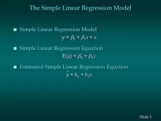
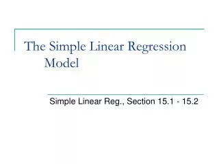
Simple Linear Regression: The Basic Mathematical Model • Regression is based on the concept of the simple proportional relationship - also known as the straight line. • Alternate Notations ! • Theory says : Y = f(x) • Mathematical form : • Statistics Literature • ei is the error (disturbance term)

Why do we include a Disturbance term? • Predicting complete system behavior in research is almost impossible. • (Unlike the models in Maths/Physics..laboratory experiments) • So we must add a component to adjust or compensate for the errors in prediction. • The disturbance term can capture a number of features: - We always leave out some determinants of yt - There may be errors in the measurement of yt that cannot be modelled. - Random outside influences on yt which we cannot model

Linear Regression:the Linguistic Interpretation • In general terms, the linear model states that the dependent variable is proportional to the value of the independent variable. • Thus, if we state that some variable Y increases in direct proportion to some increase in X, we are stating a specific mathematical model of behavior - the linear model. • Hence, if we say that the crime rate goes up as unemployment goes up, we are stating a simple linear model.

The Mathematical Interpretation: Meaning of the Regression Parameters • a = the intercept • the point where the line crosses the Y-axis. • (the value of the dependent variable when all of the independent variables = 0) • b = the slope • the increase in the dependent variable per unit change in the independent variable (also known as the 'rise over the run')

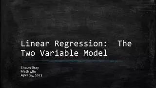
Simple Regression • For simplicity, say there is only one independent variable. This is the situation where y depends on only one x variable. • Examples of the kind of relationship that may be of interest include: • How surface finish vary depth of cut in machining • Measuring the long-term relationship between stock prices and dividends. • The number of cars sold as a sole function of its price.

Generalising the Simple Model to Multiple Linear Regression • Before, we have used the model ; t = 1,2,...,T • But, what if our dependent (y) variable depends on more than one independent variable? For example the number of cars sold might conceivably depend on 1. the price of cars 2. the price of public transport 3. the price of petrol 4. the extent of the public’s concern about global warming • Similarly, surface finish might depend on several factors. • Having just one independent variable is no good in this case - we want to have more than one x variable. It is very easy to generalise the simple model to one with k-1 regressors (independent variables).

Multiple Linear Regression :Interpretation • Multiple Linear Regression : Several Independent Variables • Interpretation of αi : • For one unit change in Xi, the mean change in Yiafter allowing for all other factors.

Determining the Regression Coefficients • So how do we determine what and are? • Choose andso that the (vertical) distances from the data points to the fitted lines are minimised (so that the line fits the data as closely as possible):

Ordinary Least Squares • The most common method used to fit a line to the data is known as OLS (ordinary least squares). • What we actually do is take each distance and square it (i.e. take the area of each of the squares in the diagram) and minimise the total sum of the squares (hence least squares). • Tightening up the notation, let yt denote the actual data point t denote the fitted value from the regression line denote the residual, yt -

Actual and Fitted Value • Graphical illustration

How OLS Works • So min. , or minimise . This is known as the residual sum of squares. • But what was ? It was the difference between the actual point and the line, yt - . • So minimising is equivalent to minimising with respect toand . • Why one has to square the error terms …can’t we minimise the sum of errors itself?

Why squared error? • Because: • (1) the sum of the errors expressed as deviations would be zero as it is with standard deviations, and • (2) some feel that big errors should be more influential than small errors. • Therefore, we wish to find the values of a and b that produce the smallest sum of squared errors.

Linearity • Linear model means….which is linear in the parameters (and ). It does not necessarily have to be linear in the variables (y and x). • Linear in the parameters means that the parameters are not multiplied together, divided, squared or cubed, etc. • Some models can be transformed to linear ones by a suitable substitution or manipulation, e.g. the exponential regression model • Then let yt= ln Ytand xt=ln Xt

The Assumptions Underlying the Classical Linear Regression Model (CLRM) • The model which we have used is known as the classical linear regression model. • We observe data for xt, but since yt also depends on ut, we must be specific about how the ut are generated. • We usually make the following set of assumptions about the ut’s (the unobservable error terms): • Technical NotationInterpretation 1. E(ut) = 0 The errors have zero mean 2. Var (ut) = 2 The variance of the errors is constant and finite over all values of xt 3. Cov (ui,uj)=0 The errors are statistically independent of one another 4. Cov (ut,xt)=0 No relationship between the error and corresponding x variate

Expressing Multiple Linear Regression Model • We could write out a separate equation for every value of t:

Testing Multiple Hypotheses: The F-test • We used the t-test to test single hypotheses, i.e. hypotheses involving only one coefficient. But what if we want to test more than one coefficient simultaneously? • We do this using the F-test. The F-test involves estimating 2 regressions.

Calculating the F-Test Statistic • The test statistic is given by where URSS = RSS from unrestricted regression RRSS = RSS from restricted regression m = number of restrictions T = number of observations k = number of regressors in unrestricted regression including a constant in the unrestricted regression (or the total number of parameters to be estimated).

Goodness of Fit Statistics • We would like some measure of how well our regression model actually fits the data. • We have goodness of fit statistics to test this: i.e. how well the sample regression function fits the data. • The most common goodness of fit statistic is known as R2. One way to define R2 is to say that it is the square of the correlation coefficient between y and . • For another explanation, recall that what we are interested in doing is explaining the variability of y about its mean value, , i.e. the total sum of squares, TSS: • We can split the TSS into two parts, the part which we have explained (known as the explained sum of squares, ESS) and the part which we did not explain using the model (the RSS).

Defining R2 • That is, TSS = ESS + RSS • Our goodness of fit statistic is • But since TSS = ESS + RSS, we can also write • R2 must always lie between zero and one. To understand this, consider two extremes RSS = TSS i.e. ESS = 0 so R2= ESS/TSS = 0 ESS = TSS i.e. RSS = 0 so R2= ESS/TSS = 1

The Limit Cases: R2 = 0 and R2 = 1

Problems with R2 as a Goodness of Fit Measure • There are a number of them: 1. R2 is defined in terms of variation about the mean of y so that if a model is reparameterised (rearranged) and the dependent variable changes, R2 will change. 2. R2 never falls if more regressors are added. to the regression, e.g. consider: Regression 1: yt = 1+ 2x2t + 3x3t + ut Regression 2: y = 1 + 2x2t + 3x3t+ 4x4t + ut R2 will always be at least as high for regression 2 relative to regression 1. 3. R2 quite often takes on values of 0.9 or higher for time series regressions.

Adjusted R2 • In order to get around these problems, a modification is often made which takes into account the loss of degrees of freedom associated with adding extra variables. This is known as , or adjusted R2: • So, if we add an extra regressor, k increases and unless R2 increases by a more than offsetting amount, will actually fall.

Regression Examples Production Function Analysis Energy Efficiency Modeling Assumptions in Regressions

A brief overview of the Linear regression model By