Download
1 / 15
150 likes | 158 Vues
Parameter, Statistic and Random Samples. A parameter is a number that describes the population. It is a fixed number, but in practice we do not know its value. A statistic is a function of the sample data, i.e., it is a quantity

E N D
Parameter, Statistic and Random Samples • A parameter is a number that describes the population. It is a fixed number, but in practice we do not know its value. • A statistic is a function of the sample data, i.e., it is a quantity whose value can be calculated from the sample data. It is a random variable with a distribution function. • The random variables X1, X2,…, Xn are said to form a (simple) random sample of size n if the Xi’s are independent random variables and each Xi has the sample probability distribution. We say that the Xi’s are iid. week1
Example • Toss a coin n times. • Suppose • Xi’s are Bernoulli random variables with p = ½ and E(Xi) = ½. • The proportion of heads is . It is a statistic. week1
Sampling Distribution of a Statistic • The sampling distribution of a statistic is the distribution of values taken by the statistic in all possible samples of the same size from the same population. • The distribution function of a statistic is NOT the same as the distribution of the original population that generated the original sample. • Probability rules can be used to obtain the distribution of a statistic provided that it is a “simple” function of the Xi’s and either there are relatively few different values in he population or else the population distribution has a “nice” form. • Alternatively, we can perform a simulation experiment to obtain information about the sampling distribution of a statistic. week1
Markov’s Inequality • If X is a non-negative random variable with E(X) < ∞ and a >0 then, Proof: week1
Chebyshev’s Inequality • For a random variable X with E(X) < ∞ and V(X) < ∞, for any a >0 • Proof: week1
Law of Large Numbers • Interested in sequence of random variables X1, X2, X3,… such that the random variables are independent and identically distributed (i.i.d). Let Suppose E(Xi) = μ , V(Xi) = σ2, then and • Intuitively, as n ∞, so week1
Formally, the Weak Law of Large Numbers (WLLN) states the following: • Suppose X1, X2, X3,…are i.i.d with E(Xi) = μ < ∞ , V(Xi) = σ2 < ∞, then for any positive number a as n ∞ . This is called Convergence in Probability. Proof: week1
Example • Flip a coin 10,000 times. Let • E(Xi) = ½ and V(Xi) = ¼ . • Take a = 0.01, then by Chebyshev’s Inequality • Chebyshev Inequality gives a very weak upper bound. • Chebyshev Inequality works regardless of the distribution of the Xi’s. • The WLLN state that the proportions of heads in the 10,000 tosses converge in probability to 0.5. week1
Strong Law of Large Number • Suppose X1, X2, X3,…are i.i.d with E(Xi) = μ < ∞ , then converges to μ as n ∞ with probability 1. That is • This is called convergence almost surely. week1
Central Limit Theorem • The central limit theorem is concerned with the limiting property of sums of random variables. • If X1, X2,…is a sequence of i.i.d random variables with mean μ and variance σ2 and , then by the WLLN we have that in probability. • The CLT concerned not just with the fact of convergence but how Sn/n fluctuates around μ. • Note that E(Sn) = nμ and V(Sn) = nσ2. The standardized version of Sn is and we have that E(Zn) = 0, V(Zn) = 1. week1
The Central Limit Theorem • Let X1, X2,…be a sequence of i.i.d random variables with E(Xi) = μ < ∞ and Var(Xi) = σ2 < ∞. Let Then, for - ∞ < x < ∞ where Z is a standard normal random variable and Ф(z)is the cdf for the standard normal distribution. • This is equivalent to saying that converges in distribution to Z ~ N(0,1). • Also, i.e. converges in distribution to Z ~ N(0,1). week1
Example • Suppose X1, X2,…are i.i.d random variables and each has the Poisson(3) distribution. So E(Xi) = V(Xi) = 3. • The CLT says that as n ∞. week1
Examples • A very common application of the CLT is the Normal approximation to the Binomial distribution. • Suppose X1, X2,…are i.i.d random variables and each has the Bernoulli(p) distribution. So E(Xi) = p and V(Xi) = p(1- p). • The CLT says that as n ∞. • Let Yn = X1 + … + Xn then Yn has a Binomial(n, p) distribution. So for large n, • Suppose we flip a biased coin 1000 times and the probability of heads on any one toss is 0.6. Find the probability of getting at least 550 heads. • Suppose we toss a coin 100 times and observed 60 heads. Is the coin fair? week1
Sampling from Normal Population • If the original population has a normal distribution, the sample mean is also normally distributed. We don’t need the CLT in this case. • In general, if X1, X2,…, Xn i.i.d N(μ, σ2) then Sn = X1+ X2+…+ Xn ~ N(nμ, nσ2) and week1
Example week1